Brief Note on a Scalar Quantum Field with Finite Lifetime in a Lorentz Invariant Non Rectangular Euclidean Space

http://dx.doi.org/10.4236/jmp.2014.514135

Brief Note on a Scalar Quantum Field with

Finite Lifetime in a Lorentz Invariant

Non-Rectangular Euclidean Space

Carmen Tornow

Institute of Planetary Research, DLR, Berlin, Germany Email: [email protected]

Received 17 April 2014; revised 14 May 2014; accepted 11 June 2014

Copyright © 2014 by author and Scientific Research Publishing Inc.

This work is licensed under the Creative Commons Attribution International License (CC BY).

http://creativecommons.org/licenses/by/4.0/

Abstract

A not necessary rectangular Euclidean space (NoNRES) is constructed, in which one obtains a gen-erally Lorentz invariant scalar product for the low energy sector (LES). This sector is defined for energies below the Planckian limit. If the energy is zero, the NoNRES becomes rectangular and due to the Lorentz invariance, it is applicable for the complete LES of the theory. In contrast to the usual Minkowski space the metric of the NoNRES depends on the kinetic energy of the observed quantum particles. It is assumed that this metric may be useful to derive the scattering cross-sec- tion of the corresponding quantum field theory. This assumption is related to the occurrence of divergent loop momentum integrals caused by including the infinite energy range above the Planckian limit (high energy sector or HES). Due to its energy dependence, the metric in both en-ergy sectors differs. In the HES, it depends on the effective dimension of the NoNRES. This de-pendency results from fluctuations of the space-time above the Planckian limit. Even if they are not part of the theory (as they would be in quantum gravity), these fluctuations should not be ig-nored. The effective dimension decreases if the energy of the considered particle increases. Since this is true for the HES only, the ultraviolet divergences of loop integrals seem to vanish without distorting the results of the LES. The mechanism is illustrated by calculating the tadpole integral occurring for a simple self-interacting scalar quantum field (with the Higgs mass as example). One obtains a finite contribution for the integral and consequently for the lifetime of the scalar particle.

Keywords

Lorentz Invariance, Scalar Field, Renormalisation, Lifetime

1. Introduction

because of short-distance interactions between the elementary particles. These interactions are considered in the high energy range of loop-momentum integrals. A well-known example for this behavior is the one loop-mo- mentum integral of the scalar QFT with a ϕ4 potential term to simulate self-interacting. Although, this theory must be seen as an artificial test model, we know that a scalar field is related to the Higgs boson [1] [2]. If one assumes a very small coupling constant for the ϕ4 potential, the dressed propagator ∆(x1, x2) is given by the

one-loop approximation and consists of the free field propagator D(x1, x2), and the tadpole diagram (Figure1).

An analysis of the momentum integral corresponding to the tadpole diagram shows that its divergence degree is +2. In order to calculate the corrected mass and lifetime of the self-interacting scalar field a regularization and renormalization procedure is needed. In general, the divergences in loop-momentum integrals originate from the fact, that special QFTs, e.g. quantum electrodynamics, are low energy approximations of a complete theory of all possible quantum particle interactions, including gravity [3]. In this study it is asked whether there is chance to simplify the regularization and renormalization procedure. As a first step to seek an answer to this question, the upper dressed propagation operator defined in Figure1 is computed with a modified method. This method requires a split of the integration range using the Planckian mass, mP =EP c2 where EP = 1.22 × 1019 GeV is the Planck energy. The related split value is kP =

(

m cP 

)

2. Accordingly, one gets for the spatial frequency k = 2π/λ or if we consider the particle masses of real and virtual particles k = 2πl where l is the inverse Compton length l = m0⋅c/ħ,

• a low energy sector (LES) with k2<kP2, i.e. Lorentz invariance of measurable (scalar) values, and

• a high energy sector (HES) with k2≥kP2=

(

m cP 

)

2, i.e. Lorentz symmetry is broken.

Actually, between the energy sector of standard QFT and the HES an appropriate transition region might exist, since it is speculated that the effects related to the violation of Lorentz invariance (e.g. polarization independent refractivity [4]) can already be detected at energies much lower than EP = mPc2. Nonetheless, it will be shown in section 3 that for the simple scalar quantum field a sharp separation works well.

Because an interval split is useless if one integrates over both energy intervals with the same method, an inte-gration measure needs to be derived that differs between LES and HES. This measure shall reflect the lower re-trievable information content of the HES compared to the LES. The next two sections explain how this measure is derived and implemented mathematically. In Section 4, the modified method of computing loop integrals is applied to the tadpole integral illustrated in Figure1. Lastly, the applicability of this integration method is dis-cussed and further steps to establish this technique are outlined.

2. Invariance of Lorentz Transformation in the Non-Rectangular Euclidean Space

It is assumed that the integration measure directly related to the geometry of Minkowski space (MS) may not be appropriate for the calculation of the high energy range of momentum integrals. Therefore, an alternative, Lor-entz invariant, geometry is constructed. It turns out that a non-rectangular space with Euclidean signature and an energy dependent angle between its space and time axes can be used. This non-rectangularity is useful to obtain an energy dependent integration measure. In this space, which is abbreviated by NoNRES (see section 3), one has general transformations given by

(

)

(

)

(

)

0 0 0

0 0 0

and ( )

and .

j j j i j i j

j j j i j i j

x x x x x x

x x x x x x

ω σ ω σ

ω σ ω σ

′= − ′= −

′ ′ ′ ′

= + = + (1)

between an inertial system Σ moving with the velocity v = Vjej and an inertial system Σ‘ moving with a velocity j j

V

′= ′

v e . The index j is arbitrary but fixed. Further one sets x0=ct≠x0′=ct′, xj ≠x′j, xk =xk′ for k ≠ j. As for the MS the scalar product of vector x=

(

x x x x0, 1, 2, 3

)

T is Lorentz invariant, i.e.,

with

x g_α αβx_β =x g_µ′ ′µνx_ν′ x_µ′ =N xα_{µ α} (2)

x1 x2 x1 x2

x1 x2

where the matrix Nαµ describes the Lorentz transformation (LT) and gαβ (g′µν) is the metric tensor in the

NoNRES. From Equation (2) we obtain

and .

gαβ =N gµα ′µνNνβ N Nαµ να =δνµ (3)

The parameter σj depend on the velocity ratios β =j Vj c and β ′j =Vj′ c where j = 1, 2, 3 is arbitrary but fixed. If one assumes for σj and ωj a relation typical for the LT, all the non-zero elements of Nαµ can be written

according to Equation (1) in the following way

1 2

0 0 2

0 , 1, 0 where 1 and .

j k j

j j k j j j j j

N =N =ω N = N =N = −σ ω ω = −σ − k≠ j (4)

All off-diagonal elements of the metric g0j

( )

g′0j in the NoNRES are related to the angle between the axis xj

( )

x′j and x0

( )

x0′ , which is influenced by the ratio βj

( )

β ′j . Based on these assumptions one obtains for the elements of gµν

00 1 0 0 1 2

, 1, where 1 and .

jj kk j j

j j j j j

g =g =λ− g = g =g = −ρ λ− λ = −ρ k≠ j (5)

The equivalent approach follows for the metric g'µν in Σ' using the coefficients ρ′j and λ′j. When Σ is an in-ertial system for a resting body its metric gµν = δµν with δµν = 1 if µ = ν and δµν = 0 if µ≠ν. An expression that relates ρj and ρ′j to σj can be derived inserting the Equations (4) and (5) into Equation (3):

( )

2

( )

2 2

( )

2

( )

2 2

0 0 0 0 0 0 0 0

0 0 ₂ 0 0 ₂

1 1

2 and 2 .

1 1

j j

j j j j j j j j

j j

N ρ N N N ρ ρ N N N ρ N ρ ρ

ρ ρ

′ ′

− −

′ ′ ′

− + = − + =

− − (6)

Because the absolute value 1−σ2j occurs in Equation (4) there are two solutions for Equation (6)

(

) (

)

or ˆ

(

) (

)

.

j j j j j j j j j j j j j j

σ = ρ λ′ −ρ λ′ λ +λ′ σ = ρ λ′ +ρ λ′ λ −λ′ (7)

We note that σ <j 1 and σ >ˆj 1. The relations in Equation (7) correspond to the addition theorems of the ve-locity ratios βj and β ′j. To show this, we need to express σj and ˆσj by βj

( )

β ′j . It follows from Equation (5) that ρj = 0 and λj = 1 for a system at rest, Σ. Equation (7) simplifies to

(

)

(

)

0 0

, 1 and ˆ , 1

j j j j j j

σ ₊=ρ′ +λ′ σ ₊ =ρ′ −λ′ (8.1)

where the index 0 indicates that one inertial system, Σ, is at rest. The two plots in Figure2 present the inverse function, i.e., the curves of ρ′j and λ′j versus the parameters σj,+ and σˆj,+. It is interesting to recognize the

increase of ρ′j on the left-hand plot and the decrease of ρ′j on the right-hand plot.

This behaviour ensures that the metric given by Equation (5) is real. Now, Σ' is at rest and Σ is the inertial system for a moving body. We set ρ′ =j 0, λ′ =j 1 in Equation (7) and obtain

0.0 0.2 0.4 0.6 0.8 1.0 0 2 4 6 8 10

0.0 0.2 0.4 0.6 0.8 1.0

0.0 0.2 0.4 0.6 0.8 1.0

j λ′

j λ′

j ρ′

j ρ′

Figure 2. Influence of velocity ratio 0 , j

(

)

(

)

0 0

, 1 and ˆ , 1 .

j j j j j j

σ −= −ρ +λ σ −= −ρ −λ (8.2)

Inserting Equations (8.1) and (8.2) into the relation for σj and ˆσj in Equation (7) it can be shown that

(

0 0

) (

0 0

)

, , 1 , ,

j j j j j

σ = σ ₊+σ ₋ +σ σ_{+ −} (9)

(

0 0

) (

0 0

)

, , , ,

ˆj 1 ˆj ˆj ˆj ˆj

σ = +σ σ+ − σ ++σ − (10)

which are indeed the addition theorems of the velocity ratios known from special relativity in the MS, where parameters σ0j,+ and

0 ,

j

σ − are equal to βj and β ′j, while for

0 ,

ˆ_j

σ + and σˆ0j,− one finds ˆβj =1βj and ˆ ₁

j j

β′= β′. Note, that matrix N_αµ is identical to the LT. In addition, time- and space-like regions can be identi-fied in the NoNRES, which are related to both of the solutions in Equation (7). The first relation in Equations (7) and (9) is the addition theorem of velocities lower than c and the second relation is the addition theorem of ve-locities higher than c. The index j, that can have values between 1 and 3, gives the three matrices N_αµ

( )

j in Equation (4) that form the Lorentz group in the NoNRES. In special relativity, a fundamental parameter is the “Eigenzeit” following from the approach

(

)

2 2 2 2 2 2

0 0

ds g d dx x dx dxj 2 jd dx xj j c tde with dxk 0, k j.

µν

µ ν ρ λ

= = + − = = ≠ (11)

It agrees with the “Eigenzeit” in the MS and verifies the identity between σ0j and βj (the plus index is sup-pressed)

( )

2

2 2 0 0

dte =dt _1− σj _⇒σj =βj ≤1 (12)

Using this “Eigenzeit” the energy-mass relation can be derived. For the particle energy E we obtain

( )

( )

( )

( )

2

0 0

2

2 0

0 0 0 0 _{2 0} 2 ₀ 2

0

1 2

with and

1 1

1

j j

j j j

j j

j m c

E cm u cmω x mc λ σ ρ σ

σ σ

σ

−

= = = ≡ = =

+ +

−

 (13)

where the vector u=

(

dx0 d , dte x1 d , dte x2 d , dte x3 dte

)

is the four-velocity, and the vector p = m0u is the

four-momentum, if the particle rest mass is m0. The energy-mass relation in Equation (13) is well-known from

special relativity in the MS. Using this equation we express the metric parameter λj as

(

)

2 4 2 2 4 2

0 2 0 1

j m c E m c j

λ = − = −ρ (14)

For a particle nearly at rest with E ~ m0c2, the NoNRES becomes almost rectangular, i.e., λj ~ 1 and ρj ~ 0. From Equation (14) it is clear that the angle between the time and the relevant space axis in Σ depends on the particle energy, just as required at the beginning of this section. If the particle energy of the quantum field in-fluences the metric attached to it, the NoNRES cannot be globally an Euclidean space, Rn, where n = 4. It seems rather to be a manifold, Mn, that is locally isomorphic to Rn. The corresponding local positions in the NoNRES are infinitesimal small regions in space and time given by the interaction events between the quantum fields.

In the following section we derive the effective dimension of the NoNRES and describe the consequences of the geometry for this number. The effective dimension is a key ingredient for the desired integration measures allowing a low-weighted consideration of the high energy sector.

3. The Effective Dimension of the NoNRES

(on-shell) or another virtual particle. They cause uncertainties for the physical parameters containing expres-sions like gµνkµkν or with similar terms. Because of Equation (13) the value of ρj approaches 1 if the particle en-ergy tends to infinity. Accordingly, the angle between the space and time axis decreases to 0˚. Moreover, all the other spatial coordinate ranges are correspondingly shrunk compared to the ranges of x0 and xj, since the factor

(

)

1 2

1 2

1

j j

λ− _{= −}ρ −

tends to infinity. As a result, the information on the dynamics of the physical parameters is overwhelmed by the metric fluctuations. Due to a broken Lorentz symmetry caused by the non-continuous space-time, the non-rectangularity of the NoNRES becomes manifest in the HES. In the LES it appears to be a transformation effect which does not seriously destroy the accuracy of the theory. Consequently all scalar values can be calculated for a 4-dimensional rectangular space in the LES. In order to consider this geometrical behav-iour of our special type of space-time in its name, it is called not necessary rectangular Euclidean space. The in-formation loss for real high quality measurements (i.e. measurements with finite but sufficient accuracy) can be quantified. An appropriate measure to describe the mixing degree of quantum states is von Neumann’s entropy SN given by [6]

( )

Trace log

( )

with

N B kl k l

S φ = −k _φ φ _ φ = θ θ (15)

where ϕ is the density matrix of an ensemble of quantum mechanical states θk. Assuming that the density matrix fulfils the eigenvalue equations: φuα = eαuα, we can simplify Equation (15) an write:

( )

log

( )

with 1

N B

S φ = − Σk e_α e_α = Σe_α (16)

where eα and (uk)α are the eigenvalues and −vectors of the d × d density matrixφ. If the d eigenvalues {eα} with

α=0,d − 1 are normalized as given in Equation (16) they can be linked to the probabilities of the states θk. Then, the von Neumann entropy in Equation (16) agrees with Shannon’s entropy and the related density matrix repre-sents an ensemble of pure states. If one sets forφthe metricg of the NoNRES, Shannon’s entropy seems to be useful to derive an effective dimension, dim(g), for the NoNRES even if g in Equation (5) depends on classical observables and not on the equivalent quantum operators (compare to Equation (14)). Using the entropy in Equation (16), one computes the effective dimension dim(g) by the following expression

( )

{

( )

}

3

( )

(

( )

)

3

( )

0 0

exp _{N B} exp ln and 1

dim g S g k e_α g E e_α g E e_α g E

α= α=

 

= = − _ _ _ _  = _ _



∑



∑

(17)

where the bar indicates normalization of the eigenvalues of the metric. The notation dim[g(E)] =: dim(E) is used to underline the energy dependency of the effective dimension which is caused by the energy dependency of the metric. If dim(E) = 4, the information content of the four vector components is measurable without any loss due to the finite accuracy of the measured data. If dim(E) < 4 uncertainties resulting from measurement errors can increase up to infinity if the smallest eigenvalue approaches zero [7]. According to Equation (5) the eigenvalues of the metric in their normalized form are

( )

(

) (

)

( )

(

)

0,1 1 j 2 1 j and 2,3 j 2 1 j .

e E = ±ρ _ +λ _ e E =λ _ +λ _ (18)

If ρj = 0, i.e., λj =1, the eigenvalues are ēα = 1/4 for all α. Thus, the effective dimension dim(E) = 4 and the space-time corresponds to an rectangular Euclidian space, i.e. a coordinate system for a resting particle. For a moving particle one obtains ρj > 0, i.e., λj < 1 leading to dim(E) < 4. Inserting Equation (14) into Equation (18) gives

(

)(

)

1 1

(

)

0 0

2 2 2 1

2 1

4 2 1 1 2 1 1 2 2 1

2 2 2

Q Q

Q Q

e e Q Q

Q Q ρ λ − −  −   − + − = = + + = _ + _ + _ = = − + − − _ − _  

 _(18.1)

(

)(

)

1 1

(

)

1 1

2 2 2 1

2 1

4 2 1 1 2 1 1 2 2 1

2 2 2

Q Q

Q Q

e e Q Q

Q Q ρ λ − −  −   − − − = = − + = _ − _ + _ = = − − − − _ − _  

 _(18.2)

(

)

1

(

)

1

2 2 3 3

2

4 4 2 1 1 2 2

2 2

Q Q

e e e e Q Q Q Q

with Q q 1 2

(

E0 E

)

2

(

m c0 2 E

)

2 −

= = = (note that the x-axis in Figure 3 presents q = E/E0,) and max(Q) =

min(q) = 1. For the usual light elementary particles with masses equivalent to the GeV-energy scale, one obtains for the LES min

( )

Q =

(

m c0 2 EP

)

2, i.e.

( )

(

)

2 2 0

max q = E_P m c and therefore, ē0 ~ 1 and ēα ~ 0 for α > 0.

Next, one gets following expression for the entropy SN according to Equation (16)

( )

log

(

4

)

log

( )

log 4

( )

log 4

( )

log

( )

4 4 4

B B B

N B

k k k

S ϕ = − Σeα eα = − Σeα eα − =k − Σeα eα (16.1)

or

( )

_{( )}

_{( )}

₍

₎

(

)

2 2 1

ln 4 ln ln 2 2 1

2 4

2 2 1

ln 2 2 1 4

N B

S Q Q Q Q

Q Q Q

k

Q Q

Q Q

− + −

= − − − + −

− − −

+ × − − −

(16.2)

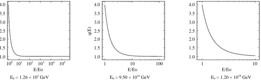
InFigure 3 the shapes of the effective dimensions, dim(E), versus the energy ratio,E/E0, for three scalar

par-ticles with different rest energiesare shown. The

( )

₄ (1 2 1 ) (1 2 1 )

2 2 1 2 2 1

Q Q Q Q

Q

dim E Q Q Q Q

Q

− − + − − − − −

= × − + − × − − − (17')

For the boundary region of LES one finds that dim E

( )

Q~0~ 1 (note: limQ→0(QQ) = 1) which corresponds to

( )

_~ ~ 1 q q

dim E ∗ where q*=EP E0 (seeFigure 3). To facilitate a comparison of the shape of dim(E) for a

particle with Higgs mass (left plot of Figure 3) with that of hypothetical super-heavy particles the other two plots are presented. The soft decrease in the middle and right plot of Figure 3results from the much higher masses of these hypothetical particles.

In contrast to the shapes of dim(E) for the super-heavy particles, the information loss calculated for the parti-cle with Higgs mass reaches its limit dim(E) = 1 for an increasing energy very rapidly. Nevertheless, a compari-son of the magnitudes of q in the three plots shows, that the different shapes become similar to each other if the number of magnitudes would be the same in all plots ofFigure 3. As a consequence, dim(E) differs between particles of different mass while dim(q) is a universal parameter. If Lorentz symmetry exists and the light speed is constant for the complete LES, the total energy of this sector cannot be higher than the Planckian limit, mPc2. Note, that in the left plot of Figure 3 the maximum energy is max(E) ~ 7 × 105 EH (with EH = mHc2) and much smaller than the maximum energy in the middle and right plots (with max(E) ~ EP). For an off-shell Higgs parti-cle the dimensional limit is reached long before the quantum fluctuations of the metric become important, the Lorentz symmetry is intact and the LT is applicable even if dim(E) ≈ 1. For off-shell super-heavy particles,

100 ₁₀1 ₁₀2 ₁₀3 ₁₀4 ₁₀5

1.0 2.0 3.0 4.0

1.5 2.5 3.5

1.0 2.0 3.0 4.0

1.5 2.5 3.5

1.0 2.0 3.0 4.0

1.5 2.5 3.5

q

(E

)

1 10 100 1 10

E/Eo

E/Eo E/Eo

[image:6.595.90.535.515.653.2]

E0 = 1.26 × 102 GeV E0 = 9.50 × 1016 GeV E0 = 1.20 × 1018 GeV

Figure 3.Loss of information, given by the dimension dim(E), between two corresponding inertial systems for a measuring device and a particle. This loss is shown for three particles with different masses in individual plots. Since dim(E) depends on the particle energy, an energy ratio, q = E/E0 is introduced. The rest energy, E0 = m0c2, in the left plot results from the

Higgs mass [1], m0 = mH. In the middle and right plot, E0 corresponds to the mass of hypothetical super-heavy particles close

especially for a particle with a mass m0 ~ mP/10 (right plot of Figure 3) the quantum fluctuations of the metric have started already while dim(E) > 1 and the transformation between inertial systems is not allowed anymore due to the broken Lorentz symmetry.

In the Introduction a transition region between the sector of the standard model is mentioned. For the simple scalar field this transition region needs not to be considered. However, the shapes of dim(E) for the super-heavy particles suggest the existence of some transition region.

4. The Interacting Scalar Particle in the NoNRES

Now, the derived integration measure is used for an interacting scalar quantum field, ϕ. We consider the 4-momentum pµ of a free scalar particle and calculate the energy-momentum relation in the NoNRES

2 2 2

0 0

g p pτν τ ν =m g u uτν τ ν =m c (19)

which leads to the Klein-Gordon operator ℵ = ∂α∂α +1 where the inverse Compton length l = m0⋅c/ħ is used to

scale the field ϕ→ϕ/l and the axes xµ → lxµ. For a self-interacting scalar field, ϕ, the action integral A[ϕ, J] is given by

[

,

]

ddim

( )

(

1

)

( )

2

[ ]

( ) ( )

A ϕ J =

∫

x g_−ϕ x ∂ ∂ +α _α ϕ x −V ϕ +J x ϕ x _ (20)

where the potential term is V[ϕ] = w/4!⋅ϕ4, J is some background field and dim is the dimension of the particle related space-time. In contrast to the MS, the metric factor g1/2 of the NoNRES, occurring in the action, gives 1. Accordingly, the path integral can be written as exp(−A/ħ), unlike exp(−iA/ħ) in the MS. The Green’s function, D(x), of a free scalar field with V[ϕ] = 0 can be calculated from

( )

( )

(

)

₍

₎

_{( )}

_{( )}

_{( )}

4 2 exp 1 d 1 1 2π dim ixk

D x k D x D x x

k i

α

α δ

ε

−

= ⇔ ∂ ∂ + = ℵ = −

− +

∫

(21)

where kν → kν/l and iε is a regularization term for the denominator if k2 = 1. The connected 2-point Green’s function (compare to the dressed propagator in Figure 1) for the weakly self-interacting field in the one-loop approximation is given by

(

1, 2

)

(

1 2

)

( )

0 d

(

1

) (

2

)

.

2

dim w

x x D x x D zD z x D z x

∆ = − +

_∫

− − (22)

The Fourier transform of Equation (22) can be expressed as

(

)

(

)

(

)

( )

(

) (

)

1 1 1 1

2 2 2 2

4 d

, 1 1 1 1 .

2 2π

dim

w k

q q q iε − q iε − k iε − q iε −

Γ − = − + + − +

_∫

− + − + (23)

Since the interaction given by Equation (20) is sufficiently weak

(

w D x

(

=0

)

1

)

one can write for Equa-tion (23)

(

)

( )

{

}

{

( )

}

2 1 ,

1 2 0 2 0

q q

q w D i ε w D

Γ − =

− + _ ⋅ℜ_ _ + − _ ⋅ ℑ_ _ (24)

where the scaled corrected mass and lifetime of the weakly self-interacting field, ϕ, result from

( )

{

( )

}

* *

1 w D 0 2 and _L 2 w D 0 .

µ = + ℜ_ _ τ = ℑ_{ } (25)

In the MS D(0) is UV divergent. However, in the NoNRES we obtain a finite expression as shown below. Considering dim = dim(E) the integral for D(0) in Equation (23), which depends on k2 only, is given by

( )

( )

(

)

( )

( )

_{( )}

( )

_{( )}

_{[ ]}

1

1 2 ₃

4

2 2

2

2 1 _{2 d}

0 d 0

1 4π 2

4π 2

dim E

dim dim E

k k i _{k k}

D k D

k i q E ε ε − − = − + = → = − + Γ

Γ _ _

where the integration range of k extends fromnullto infinity. From this equation the sought integration measure, which is ddim(E)k, can be read off. In the special case of a k2 -dependent integration function, it simplifies to

( )

₍

₎

( )1

ddimEk=ζ dim dk kdim E− . The integration range is split into the two energy sectors as explained in the In-troduction. They go from the k = 0 to Ep/m0c2 and from k = Ep/m0c2 to ∞. If the energy E< EP the physical space is modeled by a 4-dimensional rectangular Euclidean space due to the intact Lorentz symmetry and the applica-bility of the corresponding LT. If E ~ EP the LT is not allowed anymore. However, dim(E) has reached the limit dim(E) = 1 long before (see Figure3), thus, we can find a jump function for the effective dimension of the local NoNRES written as

( )

4 if P and

( )

1 if P.

dim E = E<E dim E = E≥E (27)

Consequently, we obtain for Equation (26)

( )

*

*

3

2 2 2

0

1 d 1 d

0 .

π

8π 1 1

k

k

k k k

D

k iε k iε

∞

= +

− + − +

∫

∫

(28)

Both terms are finite and give

( )

(

2

(

2

)

)

(

( )

*

)

2

2 2

1 1

0 ln 1 π arctan π 2 0.48 .

π

16π 16π

k

D k k i k i i

∗

∗ ∗

= + − − + + ≈ + (29)

Obviously, the effective dimension, dim(E), acts as a “regularization-like parameter” influencing the integra-tion result in the high-energy range. However, in contrast to usual regularizaintegra-tion procedures in the MS, dim(E) leads to a convergent result without specific normalization concepts.

Because of scaling we substitute for k* the ratio of Planckian to particle rest energy, i.e., k* = EP/m0c2. Since

the generator of the massive scalar field, ϕ, is assumed to be the Higgs particle, it results m0c2≡ mHc2 = 126 GeV

[1] [2], where mH is its mass and c is the light speed, as has already been used to calculate the shape of dim(E) presented in Figure 3. Therefore, we obtain for the corrected mass, µ*, and the un-scaled lifetime, τL, derived from Equation (25), the following results

( )

(

)

(

)

* 3

1 w D 0 2 1 1.4 10 w Js

µ _{= + ℜ ≈ + ×} − _⋅

 (30)

(

)

(

( )

)

(

)

1

(

)

_{1 2}

* 2 2

0 2 0 0 0.69 w Js ns

L L m c w D m c

τ τ − −

= =  ℑ ≈ ⋅ (31)

The coupling constant should be w ≤ 10/Js to guarantee the applicability of a first order approximation to re-arrange Equation (23). If the particle mass is not the estimated Higgs mass, but, e.g., the electron mass, we had to require a much lower upper boundary for w or Equation (24) would be invalid. The theory described by Equation (20) is true for massive scalar particles. If one likes to consider massless particles, e.g. photons, to-gether with Higgs scalars, the standard model of the electro-weak and strong interaction needs to be slightly modified to ensure its Lorentz invariance in the NoNRES.

5. Conclusions

The metric, gµν, in the NoNRES, which depends on the particle energy, E, allows to derivate an effective dimen-sion, dim(E), which is the key parameter of the integration measure ddim(E)k. In contrast to the NoNRES, the ef-fective dimension of the MS always gives dimMS(E) = 4 for all values of E, i.e., it is independent of the particle

energy. The described integration-method constructed for the NoNRES involves the high energy range of the specific QFT more appropriately than the MS, since the available information content of the observed process is considered and quantified. In addition, the NoNRES can be constructed for space-times of arbitrary dimensions. The results obtained for Equations (30) and (31) are quite reasonable. In contrast to the mass correction, the life time of the particle is mainly influenced by the result of the high energy sector, i.e., the large imaginary part of D(0) in Equation (29).

the interaction between electrons by means of photon exchange. In comparison to Equation (20), the QED action integral is more complex and contains the Abelian gauge field, Aα, and a spinor field, ψ. An extension of our in-tegration method to QED would open the access to real measurements.

Acknowledgements

The author would like to cordially thank Uwe Motschmann from the Institute for Theoretical Physics at the Technical University Braunschweig for many fruitful discussions.

References

[1] Aad, G., et al. [ATLAS Collaboration] (2012) Physics Letters B, 716, 1-29.

http://dx.doi.org/10.1016/j.physletb.2012.08.020

[2] Chatrchyan, S., et al. [CMS Collaboration] (2012) Physics Letters B, 716, 30-61.

http://dx.doi.org/10.1016/j.physletb.2012.08.02s1

[3] Delamotte, B. (2004) American Journal of Physics, 72, 170-184.

http://dx.doi.org/10.1119/1.1624112

[4] Erdmenger, J., Meyer, R. and Park, J.-H. (2007) Physical Review Letters, 98, Article ID: 261301.

http://dx.doi.org/10.1103/PhysRevLett.98.261301

[5] Gharibyan, V. (2012) Physical Review Letters, 109, Article ID: 141103.

http://dx.doi.org/10.1103/PhysRevLett.109.141103

[6] Balian, R. (2003) Séminaire Poincaré, 2, 13-27.