Munich Personal RePEc Archive
Productivity, quality and exporting
behavior under minimum quality
constraints
Hallak, Juan Carlos and Sivadasan, Jagadeesh
Univeridad de San Andres, University of Michigan
July 2008
Productivity, Quality and Exporting Behavior Under Minimum
Quality Requirements
∗Juan Carlos Hallak† and Jagadeesh Sivadasan‡
First draft May 2006
Revised July 2008
Abstract
We develop a model of international trade with two sources of firm heterogeneity: “pro-ductivity” and “caliber”. Productivity is modeled as is standard in the literature. Caliber is the ability to produce quality using few fixed inputs. While there is no quality restriction to sell domestically, exporting requires the attainment of minimum quality levels. Compared to single-attribute models of firm heterogeneity emphasizing either productivity or the ability to produce quality, our model provides a more nuanced characterization of firms’ export behavior. In particular, it explains the empirical fact that firm size is not monotonically related with export status; there are small firms that export while there are large firms that only operate in the domestic market. The model also delivers novel testable predictions. Conditional on size, exporters sell products of higher quality and at higher prices, they pay higher wages and use capital more intensively. We test these predictions using data on manufacturing establish-ments in India, the U.S., Chile, and Colombia. The empirical findings confirm the theoretical predictions.
JEL codes: F10, F12, F14,
Keywords: Productivity, quality, exports, firm heterogeneity
∗Juan Carlos Hallak thanks the National Science Foundation (grant #SES-05550190) and Jagadeesh Sivadasan
thanks the NTT program of Asian Finance and Economics for supporting this work. We also thank the Center for International Business Education (CIBE) for support. Part of the research in this paper was conducted by Jagadeesh Sivadasan as a Special Sworn Status researcher of the U.S. Census Bureau at the Michigan Census Research Data Center. This paper has been screened to ensure that no confidential data are revealed. Research results and conclusions expressed are those of the authors and do not necessarily reflect the views of the Census Bureau. We thank In ´es Armendariz, Paula Bustos, Mariana Colaccelli, Alan Deardoff, Jim Levinsohn, Diego Puga, Kim Ruhl, Eric Verhoogen and Federico Weinschelbaum for their comments and suggestions. We also thank seminar participants at the CREI (Spain), LACEA Conference (Colombia), RIEF (University of Tor-Vergata, Italy), Berkeley, UC-San Diego, UC-UC-Santa Cruz, UNIBO (Argentina), University of Michigan, Universidad de Montevideo (Uruguay), University of Oregon and UT-Austin. Santiago Sautua, Bernardo D. de Astarloa, Xiaoyang Li and Alejandro Molnar provided excellent research assistantship. All remaining errors are our own.
1
Introduction
Developing countries that have experienced rapid economic growth in the last decades have also
shown impressive export performances (World Bank 1987, 1991, 1993, 2000). The development
experiences of these countries suggest the potential importance of export growth for helping
coun-tries attain high income levels. There are various possible channels; for example, export growth
might allow firms to take advantage of unexploited economies of scale (Krueger 1998, Demiroglu
2008). Export growth could also generate productivity gains from factor reallocations, reduce
macroeconomic volatility with a more diverse exposure to shocks, and increase the absorption of
foreign technologies due to more intense interactions with the outside world (Das et al. 2007).
Since export growth is potentially an important driver of economic growth, understanding what
makes firms successful in the global marketplace is critical. Furthermore, governments increasingly
view export development as an important objective that justifies policies aimed at fostering it.1
Thus, understanding the determinants of firms’ export success can also contribute to enhancing
the effectiveness of these policies.
While work in international trade has traditionally focused on determinants of comparative
advantage at the sector level to explain patterns of trade across countries, a growing new literature
emphasizes the role played by firm heterogeneity even within narrowly defined sectors. The shifting
focus from sectors to firms reflects the understanding that, in addition to explaining countries’
export development, the identification of the determinants of firms’ export behavior is also critical
for answering the field’s core question of what determines trade patterns across countries.
In this growing heterogeneous-firm literature, a single attribute is usually the sole determinant
of firms’ ability to conduct business successfully, both domestically and abroad. This attribute
is often modeled as productivity (e.g. Bernard et al. 2003, Melitz 2003, Chaney 2008, Arkolakis
2008), or alternatively as the ability to produce quality (Baldwin and Harrigan 2007, Johnson 2008,
Verhoogen 2008, Kugler and Verhoogen 2008). Whether the single attribute is productivity or the
ability to produce quality, the models share the property that the endowment of this attribute
perfectly predicts firms’ revenue (henceforth our measure of firm size) and export status. This
property then implies a threshold firm size above which all firms export (and below which none
do).
1For example, the number of export promotion agencies in the world has tripled in the last two decades (Lederman
Although these models parsimoniously explain the salient fact that exporters tend to be large
(Clerides et al. 1998, Bernard and Jensen 1999) this prediction, common to single-attribute models,
is contradicted in the data by a large number of “anomalous” firms. Notable among them are
“born globals” – small and recently established firms with a strong export orientation (Oviatt and
McDougall 1994 and Rialp et al. 2005), and “local dynamos” – large firms that are successful in
their domestic markets but do not sell abroad (Boston Consulting Group 2008). More generally, the
models leave much of the observed relationship between firm size and export status unexplained.
As a preview of the data we will describe later in more detail, Figure 1 plots, for each of the four
countries in our sample, the fraction of exporters in each size percentile (size is adjusted by industry
mean). Violating the theoretical prediction, there are many exporters in the lowest size percentiles
as well as a substantial fraction of firms with no export activity even among the highest percentiles
of the size distribution.
In this paper, we develop a theoretical model that can explain these graphs. In addition to
firm heterogeneity in “productivity” (modeled as is typically done in the literature), we introduce
a second source of heterogeneity, “caliber”, which is the ability to produce quality using few fixed
inputs. We describe and analyze the equilibrium in a trade environment with minimum quality
requirements for export. In the presence of these requirements, firms with high productivity and low
caliber are large in size but they refrain from exporting because they find achieving the minimum
export quality excessively onerous. In turn, firms with low productivity and high caliber are active
in the export market despite being small. More generally, the model implies that export success
might depend critically on firm capabilities that are not essential for domestic success.
Although our multi-attribute model explains the non-monotonic relationship between firm size
and export status documented in Figure 1, our assessment of its empirical relevance for
characteriz-ing firms’ exportcharacteriz-ing behavior is based on testcharacteriz-ing the set of additional predictions that it generates.
These predictions are, as a whole, distinct from those generated by potential alternative
explana-tions for the relaexplana-tionship between firm size and export status.2 In particular, our model predicts
that, conditional on firm size, exporters produce higher quality and sell at higher prices. Also,
to the extent that production of quality goods requires more intensive use of skilled labor and
capital, exporters will pay higher wages and be more capital intensive. We test and find strong
support for these predictions using establishment-level data from India, the United States, Chile,
2We later discuss alternative sources of heterogeneity that could also explain the patterns observed in Figure 1
and Colombia.
The paper develops a partial-equilibrium heterogeneous-firm model with endogenous product
quality. Product quality shifts out product demand but increases marginal costs of production and
fixed costs of product development. The model embeds two sources of heterogeneity. Productivity
(ϕ) is the ability to produce output using few variable inputs. Caliber (ξ) is the ability to produce
quality with low fixed outlays. Even though caliber is the primary determinant of quality choice,
productivity also affects this choice by reducing the impact of quality on marginal costs. Therefore,
both caliber and productivity increase the firm’s optimal choice of quality.
First, we solve for the industry equilibrium in a closed economy and in a benchmark case of an
open economy with no quality requirements for export. In both cases, productivity (ϕ) and caliber
(ξ) can be combined into a single “ability” parameter η (η =η(ϕ, ξ)), such that key variables of
interest can be expressed in terms of this parameter. For example, regardless of the particular
combinations ofϕand ξ, firms with the same value ofη have identical revenue, profits, and export
status (though they choose different quality levels and charge different prices). Furthermore, the
model allows for a representation that is isomorphic to Melitz’s (2003) model. To survive in
equilibrium, firms need an ability level above a certain threshold η, while there is also a cut-off
ability level ηu that determines firms’ participation in the export market. The isomorphism with Melitz’ model is appealing as it makes the case with no export quality requirements a transparent
benchmark.
Next we analyze the full model, where we assume that to export firms are required to meet
certain minimum quality requirements.3 Although simplistic, this assumption captures a wealth of
evidence suggesting that export success is associated with firms’ ability to satisfy foreign quality
requirements.4 While different reasons, discussed later, can be invoked to justify the existence of
these export quality requirements, our aim in this paper is not to identify their particular source
3This assumption is similar to Rauch (2007), who builds a model with two quality levels in which only the high
quality good is internationally tradable.
4The international management literature widely acknowledges quality as a key requisite to access foreign markets
but rather to examine how they affect firms’ export behavior.
In the presence of minimum export quality requirements, our model delivers predictions that
depart strongly from those of single-attribute models. First, while in the closed economy firms
with identical η have equal revenue and export status, in the open economy revenue and export
status could differ even among firms with the same η. In particular, conditional onη, firms with
high caliber (and low productivity) find the quality constraint not binding while firms with low
caliber (and high productivity) might decide to remain exclusively oriented to the domestic market
to avoid a costly investment in quality upgrading. Therefore, firms of equal size (i.e. revenue) in
the closed economy could differ in size and export status after trade is liberalized. Single-attribute
models, in contrast, predict that firm size in the closed economy is a perfect predictor of export
status once the economy opens up to trade.
Second, in contrast to single-attribute models, in our model firm size is not sufficient information
to infer export status. In particular, a domestic firm that does not export might be of the same
size as another firm with a smaller volume of domestic sales but positive exports (the former firm
would have high ϕ and low ξ while the latter would have low ϕ and high ξ). Thus, variation in
export behavior within a given size percentile of the size distribution, as shown in Figure 1, can be
explained by the existence of these two types of firms.
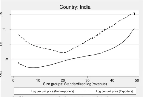
Third, conditional on firm size, the model predicts systematic differences between exporters
and non-exporters. In particular, exporters sell products of higher quality and at higher prices.
This prediction departs from those of standard models of firm heterogeneity, which predict higher
productivity and hence lower prices for exporters. It is also substantially different from results
of recently proposed single-attribute models with product quality (Baldwin and Harrigan 2007,
Johnson 2007, Kugler and Verhoogen 2008), which predict that exporters sell products of higher
quality and at higher prices unconditionally. In those models, since firm size is monotonically
related to quality, prices, and export status, there is no variation in the other variables left to
explain once size is conditioned upon.
In our model, because the export status of a firm provides relevant information about its quality
and price even after conditioning on size, in a regression framework with price as the dependent
variable, an indicator variable for export status as the independent variable, and controls for firm
size, the coefficient on the export dummy should be positive. In addition, to the extent that higher
quality products require more intensive use of skilled labor and capital, the coefficient on the export
should also be positive. These are the predictions that we take to the data.5
We employ firm-level data for manufacturing in four countries: India, the United States, Chile,
and Colombia. For India, we have a unique dataset covering all manufacturing plants for the
year 1998. In addition to data on inputs, output and exports, this dataset includes product level
information on revenue and quantities sold from which we derive prices per unit of output by
product. For the U.S., we use data from the Census of Manufactures 1997 which, like the Indian
dataset, has information on inputs, output, exports, and product level information on revenue and
quantities sold to derive per-unit prices by product. For Chile and Colombia, we have panel data
from census surveys of all manufacturing plants that employ more than 10 workers. Even though
these datasets include information on inputs, output and export but not product-level information,
we use them to obtain complementary evidence for some of our ancillary predictions.
Our analysis of the data shows that, consistent with the predictions of our model, exporters
charge higher prices, pay higher wages and are more and capital intensive, even after size is
con-trolled for. We find that the results are mostly consistent across countries and robust to using a
number of alternative specifications. We undertake a number of tests to address potential concern
about measurement error in revenue, as well as to rule out potential alternative explanations of our
results.
The goal of this paper is to propose a more nuanced characterization of the determinants of
firms’ export behavior. Thus, our empirical analysis focuses on providing evidence of its relevance.
This characterization, however, has important implications beyond what we explore here. For
example, while single-attribute models predict that the largest firms will be the ones to enter foreign
markets in response to trade liberalization, our model predicts that many of those large firms will
be unwilling to pay the required quality-upgrading costs, thus lowering the predicted magnitude
of export responses to trade liberalization. Similarly, the complex relationship between firm size
and export status stressed in our model should also affect intensive-margin versus extensive-margin
export responses to changes in trade costs (e.g. Arkolakis 2008, Chaney 2008, Ruhl 2008) as export
volumes of new entrants in the export markets are allowed to be larger than those required to
cover fixed exporting costs. More generally, we hope our model can be used as an alternative
benchmark to evaluate the effects of exchange rate fluctuations, international price movements,
trade liberalization, and other economic events or policies.
5Interestingly, some empirical papers estimate similar specifications but do not provide theoretical foundations to
Several recent papers have proposed international trade models with more than one source
of heterogeneity that can explain the lack of a one-to-one correspondence between firm size and
export status displayed in Figure 1. Alessandria and Choi (2007), Das et al. (2007) and Ruhl (2008)
build dynamic models with sunk costs of entry into the export market that deliver a cross section
of firms heterogeneous in productivity and export history. In addition, Ruhl (2008) allows for
heterogeneity in sunk export costs while Das et al. (2007) allow for heterogeneity in both sunk and
fixed exporting costs. A more closely related paper is Nguyen (2007), which also explains, among
other facts, the existence of small exporters and large domestic firms by modeling heterogeneity in
both the domestic and foreign appeal for a firm’s products. In section 5.2.1, we discuss why none
of these models can explain all the facts we document.6
The rest of the paper is organized as follows. Section 2 describes our theoretical model. Section
3 describes the data. Section 4 presents our baseline results. Section 5 performs several robustness
checks. Section 6 concludes.
2
Productivity and quality in a two-factor heterogenous-firm model
This section develops a two-factor heterogenous-firm model of industry equilibrium. In Section
2.1, we characterize the equilibrium in a closed economy. In Section 2.2, we examine the case of
a benchmark open economy with no quality constrains on exports. In Section 2.3 , we introduce
minimum quality requirements for exports and analyze the open-economy equilibrium when those
requirements are present. In Section 2.4, we analyze the factor requirements of quality production.
2.1 The closed economy
2.1.1 Demand
The model is developed in partial equilibrium. We assume a monopolistic competition framework
with constant-elasticity-of-substitution (CES) demand. The demand system here is augmented to
account for product quality variation across varieties (as in Hallak and Schott 2008):
qj =p−jσλσj−1E
P, σ >1, (1)
6Bernard, Redding, and Schott (2006) allows for heterogeneous firm-specific “ability” and product-specific
wherejindexes product varieties whilepjandλj are, respectively, the price and quality of varietyj. Since we assume that each firm produces only one variety,j also indexes firms. Eis the (exogenously
given) level of expenditure and the “price aggregator” P is defined as P ≡ R
j
p1j−σλσj−1dj. Since
σ >1, the price aggregatorP is inversely related to product prices; thus higher (lower) prices imply
a lower (higher) value of P. P can be thought of as an index of the toughness of competition in
the market. A higher P then implies a tougher competitive market.7
Product quality is modeled here as a demand shifter. It captures all attributes of a product
– other than price – that consumers value. This demand system solves a consumer maximization
problem with a Dixit-Stiglitz utility function defined in terms of quality-adjusted units of
consump-tion,qej =qjλj, and quality adjusted pricespej = λpjj. Thus, firm revenues,rj =pjqj = epjqej, can be expressed as:
rj =pej1−σ
E
P. (2)
Equation (2) indicates that larger firms are those that charge lower quality-adjusted prices.
2.1.2 Production
The model allows for two sources of firm heterogeneity. Following standard models (Melitz 2003,
Bernard et al. 2003), the first source of heterogeneity is “productivity”,ϕ, which reduces variable
production costs. Productivity enters the marginal cost function in the following form:
c(λ, ϕ) = c
ϕλ
β (3)
wherecis a constant parameter. In equation (3), marginal costs are assumed to be independent of
scale and increasing in product quality (λ). Conditional on quality, firms with higher productivity
(ϕ) pay lower variable costs.
In addition to productivity, there is a second source of heterogeneity, which we denote “caliber”
(ξ). Caliber indexes firms’ ability to develop high quality products paying low fixed costs. Fixed
costs are represented by the following function:
F(λ, ξ) =F0+
f ξλ
α (4)
whereF0 is a fixed cost of plant operation andf is a constant parameter.8 Attaining higher quality
7Note thatP1−σ is the cost-of-utility index for a CES utility function.
requires paying higher fixed costs.9 Conditional on attaining a given level of quality, those costs
are lower for high-caliber firms.
2.1.3 Firm’s optimal choice of price and quality
Firms choose price and quality to maximize post-entry profits, Π, the difference between operative
profits, Π0, and fixed costs. The first order condition with respect to price yields the standard
constant mark-up result of CES demand: pd= σσ−1ϕcλ β
d.10 Using this result, the first order condition with respect to quality yields:
λd(ϕ, ξ) =
·
1−β α
µ
σ−1
σ
¶σ³ϕ
c
´σ−1 ξ
f E P ¸1 α′ (5)
where α′ ≡α−(1−β) (σ−1). To ensure that the first order conditions identify a maximum we assume that 0< β <1, so that marginal costs are increasing in quality but not excessively fast, and
we assume that α′ > 0, so that fixed costs grow sufficiently fast with quality. Both productivity (ϕ) and caliber (ξ) have a positive impact on quality choice since they reduce, respectively, the
marginal costs and fixed costs of quality production.
Using equation (5) to solve for the optimal price, we obtain
pd(ϕ, ξ) =
µ
σ σ−1
¶α−β−(σ−1)
α′ µc
ϕ
¶α−(σ−1)
α′ ·1−β α ξ f E P ¸β α′ . (6)
Conditional on ϕ, high caliber firms sell their products more expensively because they produce
higher quality and hence have higher marginal costs. The effect of productivity on price conditional
onξ, however, is ambiguous. On the one hand, productivity lowers marginal costs and thus prices.
On the other hand, it induces the choice of higher quality levels, which in turn raises marginal
costs and prices. Whether one or the other effect dominates depends on the sign of α−(σ−1). Equation (6) shows that prices depend on the value of two parameters. Therefore, in contrast to
the predictions of quality-based models with a single heterogeneity factor (Baldwin and Harrigan
2007, Johnson 2008, Kugler and Verhoogen 2008), prices here are not monotonically related to
productivity, size, or export status.
9This approach to modeling quality production is based on Sutton (1991). It also captures the trade-offs that are
present in Yeaple (2005) and Bustos (2005), where the adoption of a superior technology requires firms to incur a fixed cost. In those models, investing in high technology shifts down the marginal cost. In a world with no export quality requirements and under specific demand assumptions, this type of investment is isomorphic to one that shifts out the demand curve.
10Subindexdis used to indicate “domestic” firms, those that only operate in the domestic market (all firms are
2.1.4 The cut-off function
Substituting the solutions for quality and price into equation (2), we obtain firm revenue:
rd(ϕ, ξ) =H
³ϕ
c
´α(σ−1) α′ µξ
f
¶α−α′ α′ µE
P
¶α α′
, (7)
H≡ ¡σ−σ1¢ (ασ−α′)
α′ ³1−β
α
´α−α′ α′
, as an increasing function of productivity (ϕ) and caliber (ξ).
From standard results of CES demand we know that operative profits equal σr. Therefore, Πd= σ1rd−Fd. Using equations (4), (5), and (7), firm profits are:
Πd(ϕ, ξ) =J
³ϕ
c
´α(σ−1) α′ µξ
f
¶α−α′ α′ µE
P
¶α α′
−F0 (8)
whereJ ≡¡σ−σ1¢
ασ α′
³
1−β α
´α α′ ³ α′
α−α′
´
. Profits are also increasing in productivity and caliber.
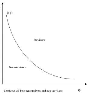
Firms remain in the market only if they can make non-negative profits (Πd≥0). Since profits depend on two variables, ϕ and ξ, this survival condition results in a cut-offfunction rather than
in a cut-offvalue:
ξ(ϕ) =f
µ
F0
J
¶ α′ α−α′ ³ϕ
c
´−α 1−β
µ
E P
¶ −α α−α′
. (9)
For each productivity level ϕ, there is a minimum caliber such that firms above this minimum
earn non-negative profits. The cut-off function ξ(ϕ) is decreasing in ϕ, highlighting a trade-off
for survival between ϕ and ξ: more productive firms can afford to be of lower caliber while high
caliber firms can afford to be less productive. The function ξ(ϕ) is displayed in Figure 2. Each
firm, characterized by a pair of draws (ϕ, ξ), can be represented in the figure by a single point.
Firms above ξ(ϕ) survive while those below this curve exit the market.
A convenient way of summarizing information about firms’ productivity and caliber is to define
their “ability”η as11
η(ϕ, ξ)≡
" ³ϕ
c
´α α′ µξ
f
¶1−β α′ #
σ−1
.
The model has the property that both revenue and profits can be expressed as functions of η
alone:12
rd(η) =ηH
µ
E P
¶α α′
, Πd(η) =ηJ
µ
E P
¶α α′
−F0. (10)
The main implication of this property is thatη is a summary statistic forϕandξ in both functions,
which depend on these heterogeneity factors only throughη. Thus firms with the sameη – such as
11We include the parameterscandf in the definition ofηonly for notation compactness.
those alongξ(ϕ) – obtain equal revenue and equal profits regardless of their particular combinations
ofη andξ. In Figure 2, this property implies that iso-ability curves are also iso-revenue curves and
iso-profit curves. Due to this property, the model can be collapsed into a one-dimensional model
iso-morphic to Melitz (2003). In particular, as in the latter model we can think of η as a single
productivity draw that determines entry-exit decisions: firms surviveiff η is above a cut-off value
η, determined so that Πd(η) = 0.13 This cut-off value satisfiesη =η(ϕ, ξ(ϕ)).
2.1.5 Free-entry and industry equilibrium
Before entering the industry, firms do not know their productivity or caliber. To learn them, they
have to pay a fixed entry costfe>0. Once they pay this cost, they drawϕand ξ from a bivariate probability distribution with density v(ϕ, ξ)>0 on the support [0, ϕ]×[0, ξ].
There is free entry into the industry. Therefore, firms pay fe and learn their productivity and caliber only if the expected post-entry profits, Π, are greater or equal than the entry cost. Since
ex-ante all firms are equal, the free entry condition imposes that
Π(P) = ϕ
Z
0
ξ
Z
ξ(ϕ,P)
Πd(ϕ, ξ, P)v(ϕ, ξ)dξdϕ=fe. (11)
Equilibrium in the industry involves finding a P that solves equation (11) (in this section we
explicitly includeP as argument of Πdand ξto emphasize its role). Finding a closed-form solution for P in equation (11) would require assuming a particular shape of the bivariate distribution
v(ϕ, ξ). Instead, we prefer to keep the analysis general and prove that a solution forP in equation
(11) exists and is unique.
Proposition 1. In the closed economy, an equilibrium in the industry exists and is unique
Proof. Since Πd(ϕ, ξ, P) andξ(ϕ, P) are continuous and differentiable inP, Π(P) is also continuous and differentiable inP. Because Π(P) is continuous, to demonstrate existence we only need to show
that this function takes the valuefe at least once. Substituting equations (8) and (9) into (11) it is easy to see that limP→0Π(P) =∞ and limP→∞Π(P) = 0. This implies that there exists at least one value of P such that Π(P) =fe.
13This property stems from the fact that the two components of the profit function, Π
0(λ) andF(λ), are particular
Since ∀(ϕ, ξ), dΠd(ϕ,ξ,P)
dP <0,application of Leibniz’s rule implies that dΠ(P)
dP <0, i.e. Π(P) is a strictly decreasing function ofP. Therefore, Π(P) takes the valuefe only once. QED
Once P is determined, we can solve for the equilibrium prices, quality levels, revenues, profits,
and cut-off values, all of which depend on P. In addition, the probability of surviving, Pin, the productivity and caliber joint density conditional on surviving, h(ϕ, ξ), and the mass of surviving
entrants,M, are also determined. The probability of surviving is given by
Pin= ϕ
Z
0
ξ
Z
ξ(ϕ,P)
v(ϕ, ξ)dξdϕ (12)
where a higher value of the cut-off functionξ(ϕ, P) implies a lower probability of successful entry.
The productivity and caliber joint density functions conditional on surviving is simply h(ϕ, ξ) = 1
Pin
v(ϕ, ξ). Finally, P can be expressed as the aggregation across productivity and (surviving)
caliber levels instead of across firms. Making appropriate substitutions we obtain
P =
Z
j
p1j−σλσj−1dj =Mα ′
αHE
α−α′ α (ηe)
α′
α (13)
where eη≡
ϕ
R
0
ξ
R
ξ(ϕ,P)
η(ϕ, ξ)h(ϕ, ξ)dξdϕis the (weighted) average ability of surviving firms. Solving
for M in equation (13) yields M = HEα′−α′αPαα′ηe−1. Since the right-hand-side of this equation
is increasing in P, in equilibrium tougher competition in the market is associated with a larger
number of entrants.
2.2 The open economy with unconstrained export quality
Before describing the full model, we examine the open-economy equilibrium in a two-country world
economy in which export quality is unconstrained. The analysis of this section provides a benchmark
for the results of the constrained case we evaluate later. Rather than analyzing differences across
countries in firm characteristics or the effects of trade liberalization, we focus on the characterization
of the equilibrium cross-section of firms in a given country. We find that, as in the closed economy,
in this “unconstrained” open economy the model can also be collapsed into a model with only one
source of heterogeneity `a la Melitz (2003).
The structure of the industry in the foreign country is analogous to that of the home country.
However, the parametersF∗
allowed to be different. The joint density function from which firms draw their productivity and
caliber is v∗(ϕ, ξ)>0, defined on the support [0, ϕ]×[0, ξ], while the (endogenously determined) price aggregator isP∗. We analyze the equilibrium cross-section of firms in the home country. The qualitative characteristics of the equilibrium in the foreign country are analogous.
In order to export, firms in the home and foreign countries need to pay fixed exporting costs,
fx and fx∗, respectively, and iceberg transport costs τ. Firms need to decide whether to become exporters or remain domestic. They choose to export if the marginal profits they would make
in the foreign market outweigh the fixed exporting costs. Exporters face CES demand in both
the domestic and the foreign markets and thus charge the same (factory gate) price at home and
abroad. The maximization problem in this case is analogous to the one described in the previous
section, except that here total demand, qw ≡ q+q∗, is the sum of domestic and foreign demand. Total demand is determined byqw =p−σλσ−1W, whereW = E
P +τ−σ E
∗
P∗. Then, exporter’s optimal
quality, revenue, and profits are given by the following expressions:
λu(ϕ, ξ) =
·
1−β α
µ
σ−1
σ
¶σ³
ϕ c
´σ−1 ξ
fW
¸1 α′
, (14)
ru(η) =ηHW
α
α′ (15)
and
Πu(η) =ηJW
α
α′ −F0−fx. (16)
Equations (14), (15), and (16) are analogous to equations (5), (7), and (8), which still determine
quality, revenue and profits for firms that do not export (the only difference is thatW substitutes
for EP). Therefore, for (unconstrained) exporters η is also a summary statistic for ϕ and ξ in the revenue and profit functions, which implies that, as in the closed economy, iso-ability curves are
also iso-revenue curves and iso-profit curves.
Define the difference in benefits between exporting and not exporting as ∆uΠ≡Πu−Πd. Using (10) and (16), this difference can also be expressed as a function of η:
∆uΠ(η) =ηJA−fx (17)
whereA=hWαα′ −¡E
P
¢α α′i
>0.
Firms choose to export if ∆uΠ(η) ≥ 0. Setting ∆uΠ(η) = 0 and solving for η, we obtain an export cut-off value, ηu, such that only firms with ability above this value export. Since η is increasing in bothϕand ξ, the cut-off value η
u also determines a cut-off function
ξ
u(ϕ) =
fx
JA
α′ α−α′
f³ϕ c
´−α(σ−1)
α−α′
which satisfies ηu = η(ϕ, ξu(ϕ)). Since η is constant along ξu(ϕ), this cut-off function is also an iso-revenue curve and an iso-profit curve.
As in Melitz (2003), there are two possible scenarios: either all surviving firms export or only
a subset of them do it. The latter case prevails if firms located on the curve ξ(ϕ) make negative
profits in the export market (Πu(ϕ, ξ(ϕ)) < 0). Hence, the existence of (purely) domestic firms is ensured with fx > (F0A)/EP
α
α′, which we assume holds for the remainder of the paper. This
assumption then implies that ξu(ϕ)> ξ(ϕ).
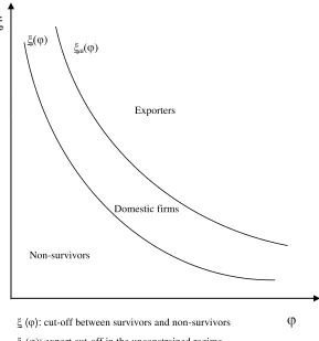
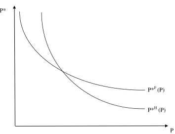
Figure 3 shows the equilibrium configuration of firms in the open economy with unconstrained
export quality. Firms with caliber below ξ(ϕ) (those with ability below the cut-off value η) exit
the market. Firms with caliber between this function and the export cut-off functionξ
u(ϕ) (those with ability between η andηu) are active in the domestic market but do not export. Finally, firms with caliber draws above ξ
u(ϕ) (those with ability aboveηu) sell domestically and also export. Since there is a one-to-one correspondence between η, revenue, and ∆uΠ, firm size (revenue) is a perfect predictor of export status. In particular, there is a cut-off size, rd(ηu), such that every firm below that size does not export while there is another cut-off size,ru(ηu), such that every firm above it exports.14 The predictions of the unconstrained model for the relationship between size
and export status are therefore stark. Figure 4 shows the fraction of exporting firms as a function
of size. As illustrated in the figure, this is a discontinuous step function. No firm with sales below
the cut-off valueru(ηu) exports while all firms with sales above that value do it. This implication is shared with all single-attribute models of firm heterogeneity.15
Finally, we note that even though revenue and profits are equal among all firms on the same
iso-ability curve η, the quality of their products is not equal. Consider the case of an exporter
located on iso-ability and iso-revenue curve ξk(ϕ), defined so that ru(ϕ, ξk(ϕ)) = k. Solving this equation for ξ and substituting the result into equation (14), we obtain:
λu(ϕ, ξk(ϕ)) =B
³ϕ
c
´−ασ−−α1′
(19)
where B is a function of constant parameters. Equation (19) shows that quality decreases along
an iso-revenue curve in ϕ×ξ space.16
14No firm has revenues in the interval“r d(ϕ, ξ
u(ϕ)), ru(ϕ, ξu(ϕ))
”
.
15Another implication, which we do not pursue further in this paper, is that since η summarizes all relevant
information determining relative size both before and after trade liberalization, the size ranking of firms should be invariant to the trade regime.
2.3 The open economy with constrained export quality
A substantial amount of evidence suggests that success in foreign markets is associated with firms’
ability to attain high levels of product quality. Brooks (2006) finds that Colombian firms in sectors
with lower quality gaps relative to G-7 countries – measured by the unit-value difference of their
exports to the U.S. – tend to export a larger fraction of their output. Verhoogen (2008) finds
that Mexican firms invest in quality upgrading in response to export opportunities created by
the Peso devaluation. Iacovone and Javorcik (2007), also working with Mexican firm-level data,
find that firms increase their average prices two years before they start exporting, which suggests a
process of quality upgrading in preparation to export. Alvarez and Lopez (2005) find similar results
focusing on investment outlays, presumably targeted at quality upgrading. More direct evidence of
the existence of export quality requirements is provided by studies in international management.
Based on firm-level surveys both in developed and developing countries, those studies document
firms’ need to upgrade quality as a crucial requirement to export [e.g. Weston 1995 (U.S.), Erel
and Ghosh 1997 (Turkey), Mersha 1997 (Africa), Anderson et al. 1999 (Canada and U.S.), Corbett
2005 (9 mostly-developed countries)]. Policy-oriented research also emphasizes the existence of
quality requirements for exports as part of a broader concern about the impact of standards on
market access (World Bank 1999, WTO 2005, Maskus et al. 2005, Chen et al. 2006).
The potential motives for the existence of export quality requirements are various. First, higher
income countries tend to consume higher-quality goods (Hallak 2006, 2007) and therefore are likely
to set higher minimum quality standards. Then, firms that on average ship their products to
higher income countries should find quality standards to be more stringent. Even if per capita
income in the export destination market is similar to that in the source country, firms may find
export quality requirements more stringent than domestic ones if quality standards are higher in
the former than in the latter countries.17 Second, transportation costs are proportionally higher
for low-quality goods (Alchian and Allen 1964, Hummels and Skiba 2004). Therefore, they can
become prohibitive below some minimum threshold. Third, export quality requirements might be
present in the form of requirements of management quality certification (e.g. ISO 9000), which
are more intensively demanded in international transactions. Since international transactions are
often conducted under severe information asymmetry problems, management quality certification
the closed economy.
17We will argue later that the much earlier implementation of ISO 9000 in the European Union than in the United
can alleviate those problems due to its quality-signaling, common-language, and conflict-setting
properties (Guler et al. 2002, Hudson and Jones 2003, Terlaak and Kind 2006, Clougherty and
Grajek 2008).
In our model, we capture the idea that entering the export market imposes more stringent
quality requirements by simply assuming that firms need to attain a minimum quality level to
export. Since in this paper we do not intend to uncover the particular source of these requirements
but rather assess their implications for the export behavior of firms, we favor a modeling choice that,
although stylized, is robust to alternative determinants of the quality constraints. Furthermore, the
predictions of the model stem more generally from the weaker condition that quality requirements
for export are more stringent than those prevailing in the domestic market.
In this section, we examine the open-economy equilibrium in a two-country world economy
with minimum quality requirements for export. The minimum is introduced as follows. In order
to export, firms need to attain at least quality level λ. The minimum is allowed to be different
across countries. Thus, it is λ∗ for firms in the foreign country that want to export to the home country. In every other respect, the “constrained” environment we analyze here is identical to the
unconstrained environment we analyzed in the previous section.
2.3.1 Characterization of the equilibrium
The main implication of the minimum export quality requirement is to force firms that would
otherwise export with qualityλu < λ to choose between upgrading their quality (relative to their unconstrained choice) or not participating in the export market. In this section, we characterize
the equilibrium in the constrained environment. As in the unconstrained case, we focus on the
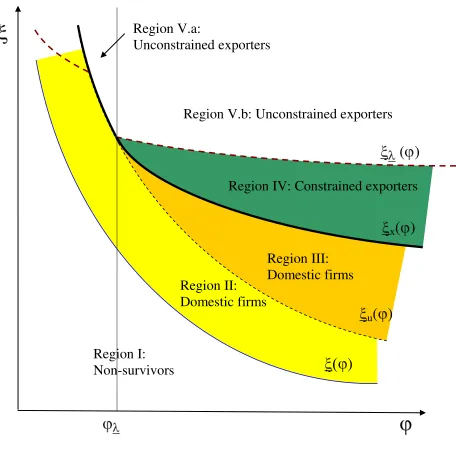
cross-sectional configuration of firm characteristics within a country, represented in Figure 5.
Firms with sufficiently low realizations of ϕorξ do not survive in the market. Those firms are
located in region I of the figure, delimited above by the cut-off function ξ(ϕ) – still determined
by equation (9). In contrast, firms located above ξ(ϕ) are either domestic or exporters. These
two types of firms are separated in the figure by the export cut-off function, ξ
x(ϕ). This function cannot be solved in closed form. To characterize it, we first need to describe the two dashed curves,
ξ
u(ϕ) and ξλ(ϕ).
The curveξu(ϕ) is the (hypothetical) export cut-off function for a single firm if the export quality restriction were removed only for that firm. By definition,ξ
ξ < ξu(ϕ). Thus, firms in this region would not export even if unconstrained in their export quality. These firms operate only in the domestic market; they do not export.
In the constrained environment, ξu(ϕ) is not the relevant export cut-off function. However, it coincides with it in part of its range. Since the unconstrained choice of quality is monotonically
decreasing inϕalongξu(ϕ) (see (19)), there exists a threshold productivity value,ϕλ, such that to its left unconstrained quality is aboveλ.18 Thus, firms located onξ
u(ϕ) with productivity ϕ≤ϕλ “spontaneously” choose quality levels above the minimum requirement. Also, as unconstrained
quality choice is increasing in ξ, unconstrained quality is higher than λ for firms located above
ξu(ϕ) on that range of productivity values. For those firms, the minimum export requirement is not binding. Thus, their export decision is still determined by the sign of ∆uΠ. This function equals zero on ξu(ϕ) and is greater than zero above it. Hence, firms located in region V.a. of the figure prefer to export.
To characterize the export cut-off function ξx(ϕ) to the right of ϕλ, we still need to describe the second dashed curve in Figure 5, ξ
λ(ϕ). This curve is the locus of firms that spontaneously choose quality levelλ. Equating (14) toλ, the expression for this iso-quality curve is19
ξλ(ϕ) =λα′f α
1−β
µ
σ−1
σ
¶−σ³
ϕ c
´−(σ−1)
W−1. (20)
Comparing equations (20) and (18), we can check that these two curves coincide atϕλandξλ(ϕ)>
ξu(ϕ) to the right of ϕλ. Since firms located aboveξλ(ϕ) spontaneously satisfy the export quality requirement, their export decisions are also governed by the sign of ∆uΠ. Thus, firms in region V.b, whereξ ≥ξλ(ϕ)> ξu(ϕ) also prefer to export.
Firms located betweenξ
u(ϕ) andξλ(ϕ) would find it profitable to sell abroad absent the export quality requirement. However, in the presence of the constraint they are forced to upgrade the
quality of their products if they wish to export. These firms need to decide whether to invest
additional resources in attaining the minimum export quality or keep their operations domestic. In
case they export, their quality isλ. In that case, marginal cost is ϕcλβ and price ispc(ϕ) = σ−σ1ϕcλβ (subindexc is used to denote “constrained” firms). Revenue and profits are, respectively,
rc(ϕ) =
µ
σ−1
σ ϕ
c
¶σ−1
λα−α′W (21)
Πc(ϕ, ξ) = 1
σ
µ
σ−1
σ ϕ
c
¶σ−1
λα−α′W −f
ξλ
α−f
x−F0.
18The expression forϕ
λcan be obtained using equations (14) and (18) to solve forϕinλu(ϕ, ξ
u(ϕ)) =λ. 19The iso-quality curve is discontinuous at ϕ
λ. To the left of ϕλ, its expression is analogous to equation (20),
except that E
Since ξ does not affect quality choice for constrained exporters, marginal cost, price, and revenue
do not depend on the value of this heterogeneity factor. Profits, however, depend onξ since firms
with higher caliber find it less costly to attainλ. Also, as firms need to deviate from their optimal
(unconstrained) choice of quality, it is easy to establish that Πc(ϕ, ξ)≤Πu(ϕ, ξ).
Define the difference in benefits between exporting and not exporting as ∆Πc ≡ Πc(ϕ, ξ)− Πd(ϕ, ξ). This difference can be written as
∆Πc(ϕ, ξ)≡ 1
σ
µ
σ−1
σ ϕ
c
¶σ−1
λα−α′W −f
ξλ
α−f x−J
³ϕ
c
´α(σ−1) α′ µξ
f
¶α−α′ α′ µE
P
¶α α′ .
The export cut-off functionξx(ϕ) is implicitly defined by the equation ∆Πc(ϕ, ξx(ϕ)) = 0. Even though we cannot solve forξ
x(ϕ) in closed form, we can characterize its slope and bound its location. First, ∆Πc(ϕ, ξ) is continuous and strictly increasing in its two arguments. Hence, by application of the implicit function theorem, ξ
x(ϕ) is continuous and decreasing inϕ. Second, we want to show that the export cut-off function is located between ξu(ϕ) and ξλ(ϕ). Note that ∆Πc(ϕ, ξu(ϕ)) < ∆Πu(ϕ, ξu(ϕ)) = 0. Therefore, firms located on ξu(ϕ) strictly prefer not to export. Also note that, since the export restriction is (just) not binding for firms located onξλ(ϕ), ∆Πc(ϕ, ξλ(ϕ)) = ∆Πu(ϕ, ξλ(ϕ))>0. Therefore, firms located alongξλ(ϕ) strictly prefer to export. Combining these two results, the continuity of ∆Πc(ϕ, ξ), and the fact that this function is strictly increasing in ξ, we can establish that ∀ϕ > ϕλ:ξu(ϕ)< ξx(ϕ)< ξλ(ϕ).
The export cut-off function ξx(ϕ) separates the last two regions of Figure 5. Firms located between ξ
u(ϕ) and ξx(ϕ) find that upgrading quality to satisfy the export requirement is too onerous. Those firms, located in region III, remain domestic. In contrast, firms located between
ξ
x(ϕ) and ξλ(ϕ), in region IV, upgrade their quality to meet the export requirement. Firms in region IV become constrained exporters.
In the case of the foreign country the analysis is analogous. In Appendix 1 we prove existence
and uniqueness of the equilibrium in this world economy.20
2.3.2 Firm size and export status
The existence of a minimum export quality requirement breaks the sufficiency of η for predicting
firm size (revenue) while it also breaks the sufficiency of size for predicting export status. In Figure
6, we add three representative iso-revenue curves,r1, r2,andr3, to the equilibrium configuration of
20A particular case of the proof, withλ=λ∗= 0, proves equilibrium existence and uniqueness in the unconstrained
firms displayed in Figure 5. First,r1represents a set of iso-revenue curves fully located in region II.
These curves can be derived from equation (10) and contain only domestic firms. Along the curves,
the value ofη is constant and is also a sufficient statistic for revenue, as in the unconstrained case.
Identical characteristics are shared byr2, which represents a set of iso-revenue curves fully located
in region III.
Iso-revenue curve r3 requires more careful analysis. Its upper-left portion is located in region
V. On this part ofr3, firms export and have identicalη. Since quality decreases along the curve, at
point A quality reaches the minimum levelλ. From A,r3 goes straight down to point B, which is
located onξx(ϕ). Since firms on this segment all produce qualityλand have the same productivity
ϕ, their marginal costs, price, and revenue are also equal. At pointB there is a discontinuity inr3,
which reappears further to the right — in region III — as shown in the figure. This last portion
of the iso-revenue curve contains only domestic firms, which attain revenue level r3 compensating
their lack of exports with more voluminous sales in the domestic market. Note that, as they have a
higherη, in an unconstrained environment they would have been larger than firms on the upper-left
portion ofr3. The limit case of this set of iso-revenue curves isrx, which is the minimum possible revenue for an exporter.
The distinct feature of iso-revenue curver3 is the fact that it includes both exporters and
non-exporters. Therefore, its level is not sufficient information to predict the export status of firms on
the curve. This implies that, in contrast to the unconstrained case and the predictions of
single-attribute models of firm heterogeneity, the relationship between firm size and fraction of exporters
is not a step function as in Figure 4. Here, the fraction of exporters is strictly between 0 and 1 for
a broad range of revenue levels. This prediction is consistent with the evidence presented in Figure
1, which shows the presence of both exporters and non-exporters at most revenue levels.21 An
additional prediction that contrasts with single-attribute models and our unconstrained case, but
which we do not test in this paper, is that firm size in the closed economy does not perfectly predict
export status in the open economy. While firm size in the closed economy is solely determined by
the value ofη, in the open economy firms with equalη need not have equal size.
21Even though the theory predicts this fraction to be 0 for sufficiently low revenue and 1 for sufficiently high revenue
2.3.3 Testable predictions
In addition to explaining the simultaneous existence of exporters and non-exporters with equal
revenue, the model predicts that, conditional on being located on the same iso-revenue curve, these
two type of firms will display systematic differences in quality levels and prices. Consider any
exporter on such a curve, characterized by the pair of draws (ϕx, ξx). Denote by λx(ϕx, ξx) her optimal choice of quality. This exporter might be either constrained or unconstrained in her choice
of quality. In the case of an unconstrained exporter, λx(ϕx, ξx) = λu(ϕx, ξx). In the case of a constrained exporter, λx(ϕx, ξx) = λ. Now consider any domestic firm on the same curve with draws (ϕd, ξd). In this case, optimal quality is λd(ϕd, ξd). The following proposition establishes that, for firms on the same iso-revenue curve, exporters produce higher quality than non-exporters.
Proposition 2. Conditional on size (total revenue), quality is higher for exporters than for
do-mestic firms:
∀r, λx(ϕx, ξx)|r=r > λd(ϕd, ξd)|r=r (22)
In turn, (22) implies the weaker statement:
∀r, E[λx(ϕx, ξx)|r=r]> E[λd(ϕd, ξd)|r=r]. (23)
For r < rx, since none of the firms exports this proposition is vacuous. Proof. See Appendix 2.
This result can be verified by visual inspection of Figure 6. Exporters are either firms located
between pointsAand B, in which case they produce qualityλ, or firms located aboveA, in which
case they produce quality aboveλ. Instead, non-exporters are located to the right ofC, and thus
produce quality below λ. In particular, exporters are firms with relatively high caliber and low
productivity while non-exporters are firms with low caliber but high productivity.
Since quality is unobservable, our empirical investigation relies on corollaries of Proposition 2.22
22Our model can potentially deliver testable predictions about reallocation of resources following trade
Corollary 1 states that, holding size constant, exporters charge higher prices than non-exporters:
Corollary 1. Conditional on size, exporters charge higher prices than domestic firms:
∀r, px(ϕ, ξ)|r=r > pd(ϕ, ξ)|r=r. (24)
In turn, (24) implies the weaker statement:
∀r, E[px(ϕ, ξ)|r=r]> E[pd(ϕ, ξ)|r=r]
Proof. With CES demand, ri = piqi = p1i−σλiσ−1Di, where Di = PE if i = d and Di = W if
i=x={u, c}. Solving forpi, we obtainpi=r
1 1−σ
i λiD
1 σ−1
i . On the same iso-revenue curve,rx =rd. Then, sinceW > EP and λx > λd(Proposition 2), Corrollary 1 easily follows. QED
Proposition 2 is the basis of our empirical investigation while Corollary 1 is the main empirical
prediction. These are novel results in the literature. Even though several models of firm
hetero-geneity with quality differentiation predict that exporters produce higher quality and sell at higher
prices than non-exporters (e.g. Baldwin and Harrigan 2007, Johnson 2007, Verhoogen 2008, Kugler
and Verhoogen 2008), those models do not deliver these resultsholding size constant. Conditional
on size, they predict that all firms have the same export status: either all are exporters or they are
non-exporters. Here non-exporters can achieve the same revenue level as exporters by producing
higher quantities, which they sell at lower prices because of their higher productivity. However,
their lack of caliber makes them unable to reach the quality standards of foreign markets. Despite
their high productivity and large size in the domestic market, they remain local.
2.4 Factor input requirements of quality production
The model developed so far assumes that both fixed and variable costs of production increase with
the level of quality. Since this is a partial equilibrium model, we have left the source of those costs
unmodeled so far. In this section, we model the fixed and variable costs of producing quality in
more detail following an approach that partially draws on Verhoogen (2008). This allows us to
relate the production of quality to average wages and capital intensity.
Production requires the use of two primary factors, labor and capital. There are HL types of labor, indexed by h = 1, ...H, which earn market-determined wages wL
h. There are also HK types of capital, indexed by h = 1, ..., HK, and V vintages of each type of capital, indexed by
same type of capital are perfect substitutes and equally productive. Therefore, they earn identical
market-determined rental rate wK
h . The price of a unit of capital of type h and vintage v is phv and equals the discounted future sum of rental rates: phv =Pvt=0
wK ht
ρt , where ρt = Π
t
t′=0(1 +ρt′)
and ρt′ is the one period interest rate.
Denote by Lh the units of labor of type h, by Kh =PVv=0−1Khv the units of capital of type h hired by the firm, and defineL=PhLh and K =PhKh. Then, the average wage the firm pays is wL =
P
hwhLLh
L and the average rental is wK =
P
hwhKKh
K . Wages and rental rate gaps across types of factor inputs can be thought to reflect differences in relative productivity in an unmodeled
“numeraire” industry. In the case of labor, relative productivity is assumed to depend on skills.
To produce quality λ, a firm needs to pay average wage wL = wLλbL and average rental rate
wK =wKλbK,b
L>0,bK >0, wherewLandwK are the least expensive types of labor and capital, respectively. This requirement applies to factor inputs associated both with fixed and variable
costs. Thus, producing higher quality requires hiring more skilled and higher-paid workers and
more expensive types of capital.
The volume (quantity) of output produced does not depend on the type of inputs used in
production but only on their quantities. Output is produced using a constant returns to scale
Cobb-Douglas production function: Y =ϕLαLKαK, whereα
L+αK = 1. This production function yields the unit cost function, conditional on qualityλ, postulated in equation (3):
c(λ, ϕ) = A
ϕ
¡
wL¢αL¡wK¢αK = c
ϕλ
β
whereA= 1
ααL
L α
αK
K
,c=A¡wL¢αL¡
wK¢αK
, and β =αLbL+αKbK.
The fixed cost part of quality production is modeled in a very similar manner. Specifically, we
assume that it requires labor and capital combined in a Cobb-Douglas production function with
the same exponents: λ = [ξL′αLK′αK]1/κ.23 These quality-related fixed costs can be thought of
as expenses related to the implementation of quality control systems, worker training, or product
development.24 In addition, the firm incurs other fixed costs F
0 (such as annual maintenance
expenses or headquarter expenses) unrelated to quality. Accordingly, fixed costs, conditional on
qualityλ, are as defined in equation (4):
F(λ, ξ) = A
ξ
¡
wL¢αL¡
wK¢αK
λκ+F0 =
f ξλ
α+F
0
23Bernard et al. (2007) also assume that input shares associated with fixed and variable costs are equal.
24In this static framework, sunk and fixed costs are equivalent. In a dynamic setting, sunk costs could still be
wheref =A¡wL¢αL¡
wK¢αK
and α=κ+αLbL+αKbK.25
These assumptions, together with the results of Proposition 2, imply a systematic relationship
between factor use, quality, and size.
Corollary 2. Conditional on size, average wages are higher for exporting firms.
Proof. This corollary follows directly from the assumptions of this section and Proposition 2. In
particular, since average wages are a monotonically increasing function of quality, Proposition 2
implies that
∀r, wL(λx(ϕx, ξx))|r=r> wL(λd(ϕd, ξd))|r=r
Corollary 3. Conditional on size, capital intensity is higher for exporting firms. Capital intensity
is measured as the (value of ) capital-to-labor ratio, V KL , where V K =PHh=1PVv=1phvKhv
Proof. See Appendix 3.
Corollary 2 simply connects Proposition 2 with our assumption about labor requirements of
quality production. Exporters need to pay higher average wages because they produce higher
quality, which requires a more expensive and higher skilled composition of the labor force. Corollary
3 captures a similar effect. In this case, we note that, since a simple count of “machine units” is
meaningless, “physical” capital, as reported in firm-level statistics, cannot be treated analogously
to the count of bodies in the case of labor. In terms of our notation, we observeV K, not K. Both
Corollaries 2 and 3 can be weakened to be stated in expected values. We take these predictions to
the data in this last form.
3
Data
3.1 Data sources
Our empirical analysis utilizes establishment-level manufacturing survey data from the India, US,
Chile and Colombia. We discuss the data sources briefly below; more specific discussion of the
product level information for India and US, and the steps we took to clean the data for all four
datasets is discussed in the Data Appendix.
25From the expression forβ above, we obtain α =κ+β. In Section 2.1 (see discussion below equation 5), we
For India, we use a cross section of the Annual Survey of Industries (ASI) for the year 1997-98.
We focus on 1997-98 because the ASI data for this year includes information on exports and on
output quantities and values. This information is critical for our analysis because it allows us
to construct product level prices (unit values). Another useful feature of the data is that it has
information on whether each plant has obtained ISO 9000 certification, which can be used as a
direct proxy for quality. The ASI is a survey undertaken by a government department called the
Central Statistical Organization (CSO). It covers all industrial establishments (called “Factories”)
registered under the Factories Act employing more than 20 persons.26 The ASI frame includes two
“sectors”: the census sector and the sample sector. All factories in the census sector (employing
more than 100 workers or located in designated backward areas) are surveyed. Factories in the
sample sector are stratified and randomly sampled. Throughout our analysis, we appropriately
adjust for sampling weights (called ”multiplier”). Further details about this data can be found in
Sivadasan (2007).
For the US, we use data from the 1997 Census of Manufactures (CMF). The CMF data is
collected by the US Census Bureau as part of the quinquennial economic census. It covers all
manufacturing establishments that employs even one paid worker, and includes detailed information
on inputs and outputs at the establishment level. It has been used very extensively in microeconomic
research work in general (see e.g. survey by Bartelsman and Doms 1999), and also specifically to
examine differences between exporters and non-exporters in pioneering work by Bernard and Jensen
(1999). A detailed discussion of the Census of Manufactures data is available in LRD technical
documentation manual (1992).
The novelty in this paper with regard to CMF data is the use of SIC seven-digit product-specific
information on product quantity and product revenue to derive a per unit value or price (defined
as product revenue divided by product quantity).27 One drawback of our derived per unit value
measure is that product quantity data is unavailable for many establishments and products. In
particular, quantity information is often missing for certain products or industries where output
26The limit is lower (10 employees) for plants that use electric power for production. Some plants in the data report
less than 10 employees, apparently because some plants below the mandated limit voluntarily choose to register or because some plants that initially registered when they had more than 10 employees remain registered even after employment levels fall below the cutoff.
27A recent paper that exploits the seven-digit product level information on quantity and revenue is Foster,
units are ”not meaningful” (LRD manual, 1992). However, since our model’s predictions relate to
comparisons across establishments (firms)within industries, lack of information for entire products
or industries should not bias our results.28
Data for a large proportion (about 40%) of (largely smaller sized) plants (”AR plants”) are
collated by the census from administrative records. Many studies using census manufacturing data
exclude these observations (e.g. Syverson 2004, Bernard, Redding and Schott, 2008). Because price
data is unavailable for AR firms, our price analysis also excludes them. For the other non-price
variables, since we are interested in examining differences across the size distribution, we retain the
AR plants in the baseline analysis, but perform sensitivity checks to excluding AR plants.
We use manufacturing data for Chile and Colombia to examine predictions relating to
non-price variables, as product level revenue and quantity (and hence non-price) data is unavailable in these
datasets.
For Chile, the data we use is drawn from the annual Chilean Manufacturing Census (Encuesta
Nacional Industrial Anual) conducted by the Chilean government statistical office (Instituto
Na-cional de Estadistica). The census covers all manufacturing plants in Chile with more than 10
employees and has been conducted annually since 1979. We use data for the years 1991-96, for
which data on export activity is available. Further details about this dataset can be found in Liu
(1991) or Roberts and Tybout (1996).
Finally, data for Colombia comes from the Colombian manufacturing census for the years 1981
to 1991. As in the Chilean case, the Colombian census covers all plants with 10 or more employees.
A more detailed description of the Colombian datasets can be found in Roberts and Tybout (1996,
Chapter 10).
3.2 Definition of variables and summary statistics
Testing the predictions of our theoretical model requires data on export status, revenue, potential
proxies for quality, output price, average wage, and capital intensity (capital to labor ratio).29
Ideally, we would like to have a measure of quality that is directly consistent with λ in our
model, which affects the marginal costs and fixed costs of operations. While this ideal measure is
unavailable, in the Indian dataset each plant reports if it has obtained ISO 9000 certification. We
28In other words, our model could potentially be tested with sufficiently detailed data on a single industry or
product. In any event, we undertake a robustness tests to check if results are sensitive to including information on products where price data is sparse (see in Section 4.2.3).
discuss in Section 4.3 why the ISO 9000 quality management certification could be a good proxy
for quality (λ).
Export status is captured by a dummy variable defined to equal one for all establishments
reporting positive value of exports. Revenue is total sales by the establishment. Labor is measured
as total employment, log average wage is obtained by taking the logarithm of the ratio of total
wages to total employment, for each establishment. The variable capital, in the case of Chile,
is constructed using the perpetual inventory method. For India, US, and Colombia, capital is
measured as reported total fixed assets.
As discussed in Section 3.1 above, the datasets for India and US contain information on the
separate product lines of every establishment. This allows us to derive prices or unit values, which is
critical for testing Corollary 1. Specifically, for each product line, the dataset provides information
on sales value and quantity. The ratio of the two results in a unit value, which we use as a proxy
for price.
The price variable is defined at the product category level, so that there are multiple price
observations for each firm. Since all other data, in particular data on export value, is available
only at the establishment level, in our analysis we check robustness to different assumptions about
which product lines may be exported (see discussion in Section 4.2).
In the case of all other non-price variables (in particular, revenue, employment, average wage
and capital intensity), because the statistical unit in the Indian, Chilean and Colombian datasets
is the establishment, we define and measure these variables at the establishment level. In the
baseline analysis for the US, we adopt the same approach and define all non-price variables at the
establishment level. However, in the US data, there are well defined ownership links that allow
us to aggregate data to the firm level, and in Section 5.1, we discuss robustness of the results to
defining size and other variables at the firm level.
To mitigate influence of outliers, as discussed in the data appendix, all variables are winsorized
by 1% on both tails of the distribution.
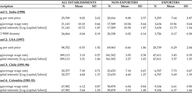
Panels 1, 2, 3 and 4 of Table 1 present summary statistics for India, US, Chile and Colombia,
respectively. In the case of India, all statistics are adjusted to account for sampling weights.
Sampling weights are not relevant for the census data of the US, Chile and Colombia, where
establishments are sampled with certainty. The nominal variables (wages and capital) for India