Global tropospheric ozone modeling: Quantifying
errors due to grid resolution
Oliver Wild1,2 and Michael J. Prather3
Received 22 August 2005; revised 2 December 2005; accepted 23 February 2006; published 9 June 2006.
[1] Ozone production in global chemical models is dependent on model resolution
because ozone chemistry is inherently nonlinear, the timescales for chemical production are short, and precursors are artificially distributed over the spatial scale of the model grid. In this study we examine the sensitivity of ozone, its precursors, and its production to resolution by running a global chemical transport model at four different resolutions between T21 (5.65.6) and T106 (1.11.1) and by quantifying the errors in regional and global budgets. The sensitivity to vertical mixing through the
parameterization of boundary layer turbulence is also examined. We find less ozone production in the boundary layer at higher resolution, consistent with slower chemical production in polluted emission regions and greater export of precursors. Agreement with ozonesonde and aircraft measurements made during the NASA TRACE-P campaign over the western Pacific in spring 2001 is consistently better at higher resolution. We
demonstrate that the numerical errors in transport processes on a given resolution converge geometrically for a tracer at successively higher resolutions. The convergence in ozone production on progressing from T21 to T42, T63, and T106 resolution is likewise monotonic but indicates that there are still large errors at 120 km scales, suggesting that T106 resolution is too coarse to resolve regional ozone production. Diagnosing the ozone production and precursor transport that follow a short pulse of emissions over east Asia in springtime allows us to quantify the impacts of resolution on both regional and global ozone. Production close to continental emission regions is overestimated by 27% at T21 resolution, by 13% at T42 resolution, and by 5% at T106 resolution. However, subsequent ozone production in the free troposphere is not greatly affected. We find that the export of short-lived precursors such as NOx by convection is overestimated at coarse
resolution.
Citation: Wild, O., and M. J. Prather (2006), Global tropospheric ozone modeling: Quantifying errors due to grid resolution, J. Geophys. Res.,111, D11305, doi:10.1029/2005JD006605.
1. Introduction
[2] Ozone is formed in the troposphere as a by-product of
the oxidation of hydrocarbons and carbon monoxide in the presence of nitrogen oxides (NOx) and sunlight [Chameides
and Walker, 1973; Crutzen, 1974]. Ozone production is dependent on precursor concentrations in a nonlinear man-ner [Liu et al., 1987;Lin et al., 1988], and much of it occurs on short timescales close to regions with high emissions of precursors. Chemical transport models (CTMs) that are used to simulate regional O3buildup need to resolve the
corre-spondingly small spatial scales involved to avoid systematic
overestimation of regional O3production due to excessive
spatial averaging of emissions [Chatfield and Delany, 1990;
Sillman et al., 1990;Jang et al., 1995a, 1995b]. However, assessing the impacts of O3 on global climate and
tropo-spheric oxidizing capacity, or of intercontinental transport of O3on regional air quality, requires use of a CTM with a
global domain. Computational constraints currently limit these global models to spatial scales of 1(about 110 km) or greater. While this is sufficient to resolve regional variations in the mean flow patterns associated with atmospheric transport, it may be insufficient to prevent the premature mixing of O3 precursors in polluted regions, the
overesti-mation of regional O3production, and the underestimation
of precursor lifetimes and export to the global troposphere. The balance between production in the polluted boundary layer and in the global troposphere is thus incorrect. This has significant implications for assessment of the impacts of surface emissions on the global environment, for example in the attribution of climate impacts due to changes in O3and
CH4from specific source regions. While global models are
not tailored to simulate the chemical processing that occurs Here
for
Full Article
1
Frontier Research Center for Global Change, Independent Adminis-trative Institution Japan Agency for Marine-Earth Science and Technology (JAMSTEC), Yokohama, Japan.
2Now at Centre for Atmospheric Science, University of Cambridge, Cambridge, UK.
3Earth System Science, University of California, Irvine, California, USA.
during the mix-down of concentrated plumes associated with urban and industrial sources, the magnitude of the errors involved must be assessed to correct for the bias in simulation of O3on regional and global scales.
[3] In this paper we explore systematically the sensitivity
of modeled O3 production to horizontal resolution with a
sequence of four nested model resolutions, and investigate whether it starts to converge over the resolutions currently employed by global CTM and climate models. Studies including subgrid scale parameterizations of urban chemis-try in regional and zonally averaged global models have demonstrated that calculated O3production is lower when
the separation between polluted and rural environments is better resolved [Sillman et al., 1990; Jacob et al., 1993;
Mayer et al., 2000]. We demonstrate convergence for a passive tracer, and then investigate the extent of conver-gence with full chemistry. Converconver-gence would allow an estimate of the error in O3production at a given resolution,
while a lack of convergence may suggest that production close to source regions is occurring at temporal and spatial scales far smaller than those resolved at the highest reso-lutions used here. Recent studies running global CTMs at different resolutions have confirmed the lower O3
produc-tion at higher resoluproduc-tion [Kentarchos et al., 2001; von Kuhlmann et al., 2003; Wild et al., 2004; Esler et al., 2004;Park et al., 2004;Krol et al., 2005], but in many of these studies the simulations at different resolutions are not directly comparable. Moreover, in comparing only two resolutions they are unable to demonstrate a systematic convergence with resolution or to quantify the errors in O3production.
[4] Testing the quality of model simulations is difficult as
O3production cannot be measured directly. Climatological
comparisons with monthly mean O3 measurements from
sonde, surface and aircraft platforms are commonly used to evaluate global CTMs [e.g., Houweling et al., 1998;Wang et al., 1998; Horowitz et al., 2003; von Kuhlmann et al., 2003; Wild et al., 2003; Hauglustaine et al., 2004] but provide only a rough indication that the seasonal behavior of O3is appropriately modeled. Case-by-case comparisons
under the correct meteorological conditions provide more information on how well stratospheric intrusions or conti-nental plumes are captured [e.g., Roelofs et al., 2003;Wild et al., 2003], but are sensitive to the simulation of meteo-rological features [e.g., Kiley et al., 2003] and do not constitute a critical test of the simulated time scales for O3formation.
[5] To provide a regional focus for this study we consider
O3production from east Asian sources in springtime. Rapid
industrial and economic development in this region make it increasingly important as a source of O3 to the global
troposphere [Berntsen et al., 1996; Carmichael et al., 1998; Jaffe et al., 1999]. In addition, measurements made during the NASA Transport and Chemical Evolution over the Pacific (TRACE-P) measurement campaign held in spring 2001 [Jacob et al., 2003] provide an extensive sampling of the chemical composition of Asian outflow and allow a detailed assessment of model performance for a wide range of chemical species.
[6] We describe the model approach taken in section 2. In
section 3 we demonstrate convergence for a passive tracer with increasing resolution. In section 4 we consider full
chemistry, and evaluate the changes in regional O3
produc-tion over east Asia with increasing resoluproduc-tion, comparing the simulations against measurements made during the TRACE-P campaign. The impacts on O3 abundance and
production on a global scale are described in section 5. In section 6 we describe the O3response to regional emissions,
exploring the balance between regional and global production for east Asian emissions. We investigate con-vergence in the O3 budget and quantify the errors due to
horizontal resolution in section 7. Conclusions are presented in section 8.
2. Model Approach
[7] This study uses the Frontier Research System for
Global Change (FRSGC) version of the University of California, Irvine (UCI) global chemical transport model (CTM) described by Wild and Prather[2000]. The model is driven by 3-hour meteorological fields generated with the European Centre for Medium-Range Weather Fore-casts (ECMWF) Integrated Forecast System (IFS) at a spectral resolution of T159 with 40 eta-levels in the vertical. These fields have been used at T21 (5.6
5.6) and T63 (1.9 1.9) resolution with 37 vertical levels in previous studies, [Wild et al., 2003, 2004; Hsu et al., 2004] and are also used here at T42 (2.8 2.8) and T106 (1.1 1.1) resolution. The different resolu-tions are run from the same T159 fields so that the dynamics are continuous from T21 to T106. The notable strengths of these pieced-forecast fields over other anal-ysis products available include their dynamical self-con-sistency, the use of integrated or averaged quantities, the range of diagnostics included, the longer spin-up to reduce analysis noise, and the 3-hour temporal resolution. [8] The performance of the model in simulating the
observed distribution and variability of O3 and its
precur-sors over east Asia has been presented in earlier studies [Wild et al., 2003, 2004]. A number of small changes have been made for the present studies, including revising the dry deposition scheme to follow that of Wesely [1989], and standardizing the emissions from biomass burning and lightning sources such that the magnitude and distribution of sources remains independent of model resolution. Lightning emissions of NOx are based on diagnosed
con-vective mass fluxes at T106 resolution, followingAllen and Pickering[2002], the vertical distribution of the source is now based on observed profiles [Pickering et al., 1998], and total emissions are normalized to 5 Tg(N)/yr. For boundary layer mixing, the previous versions of the CTM applied a simple, hourly bulk-mixing of tracers from the surface to the diagnosed mixing height. This has been replaced with a nonlocal K-profile treatment of boundary layer turbulence [Holtslag and Boville, 1993] based on the surface energy fluxes generated by the IFS model. At T106 resolution the standard 11surface emissions data are inadequate for resolving the heterogeneity of emissions, and anthropogenic emissions of NOx, CO and NMHC over east Asia are
the subgrid scale variation in emissions is used by the second-order moment advection scheme [Prather, 1986].
[9] Compared with the previously published studies, the
effect of these changes is relatively small: surface O3at high
latitudes is lower because of greater deposition, O3levels in
the tropical upper troposphere are larger because of a greater proportion of lightning NOx emissions at high altitude,
and CO is higher because of a 20% increase in east Asian industrial CO emissions in the updated emissions data set. Each of these changes brings simulated trace gas concentrations into closer agreement with TRACE-P measurements.
[10] The impact of aerosol particles on photochemistry
was not included in previous studies using the FRSGC/ UCI CTM. Aerosols may influence O3 production by
absorption and scattering of sunlight [Martin et al., 2003;
Bian et al., 2003] and by providing surfaces on which heterogeneous reactions can occur [Jacob, 2000]. The deserts and industrial regions of China are a large source of aerosol in springtime [e.g.,Duce et al., 1980], and this is known to influence regional O3production at this time
of year [Tang et al., 2003]. To include the impacts of aerosols we apply monthly mean aerosol optical depth distributions for 2001 from the Moderate Resolution Imaging Spectroradiometer (MODIS) instrument on the Terra satellite (data available from http://modis-atmos.-gsfc.nasa.gov). These optical depths are apportioned be-tween different aerosol types (sulphate, soil dust, carbonaceous aerosols and sea salt) on the basis of model-derived monthly climatologies [Tegen et al., 1997], and photolysis rates are calculated online in the CTM using Fast-J [Wild et al., 2000]. This method neglects the day-to-day variability in aerosol distributions, but includes the colocation of industrial aerosols and O3
precursors to the extent that the MODIS climatology does.
[11] The standard model simulations performed here at
four different resolutions apply the K-profile boundary layer mixing and do not use the optional aerosol climatology. These simulations are repeated, firstly with a 1-hour mixed boundary layer as used in earlier studies, and then separately with the impacts of aerosol on photolysis included. The thorough vertical mixing of surface pollutants throughout the boundary layer on a 1-hour timescale has a comparable effect to the greater horizontal mixing implicit at coarser model resolution, and leads to a similar overestimation of O3 production. In
contrast, the modification of photolysis rates due to the presence of aerosol particles generally reduces production in polluted boundary layers, altering the chemical time scales and thus the magnitude and location of production. These alternative model formulations allow the sensitivity of the convergence in O3production with resolution to be
examined. Errors in O3 production with resolution are
generally referenced to the standard T42 simulation as this is typical of current high-resolution global CTMs.
[12] We first look at the resolution error and its
conver-gence for transport processes alone using a simple, con-served tracer. The effects of resolution and mixing on O3
photochemistry are then explored using two different diag-nostic approaches. We first compare net and gross produc-tion rates over selected diagnostic regions to determine the
regional and global sensitivity of production and the impacts of resolution and mixing on the simulation of oxidation processes. We then investigate the impacts of this on O3 production from sources over a single emission
region by applying a small perturbation to emissions and following the response of O3 and its precursors over the
subsequent weeks. This allows a clear assessment of impacts on the location and evolution of O3 production
and thus on the biases due to resolution that may be expected in studies of the long-range transport of O3or of
its source attribution.
3. Convergence of Tracer Transport With Increasing Resolution
[13] The errors of a correctly formulated numerical
model solved on a grid should be in proportion to the grid resolution (generically denoted here as h). As the grid step h becomes smaller, the numerical solution converges to the correct answer. We test this convergence in CTMs with the simplified case of transport of a conserved tracer. This test case is derived from studies with the NASA Global Modeling Initiative (GMI), which has developed a modular CTM on a fast computing platform for critical evaluation of different model compo-nents [Douglass et al., 1999; Rotman et al., 2001;
Kinnison et al., 2001] and for scientific assessments (e.g., aviation impacts, greenhouse gases). One of the GMI tests involved identical simulations with both GMI and UCI CTMs using the same meteorological fields (from the Goddard Institute for Space Studies GISS-II’ model at 4 latitude by 5 longitude resolution with 23 layers [Rind et al., 1998]), boundary conditions (fossil fuel CO2 emissions [Brenkert, 1998]) and chemistry
(none). The differences in these ‘‘identical’’ simulations were large, even in comparison with the full range of different models in TransCom3 [Gurney et al., 2003]. This highlights the fact that the modeling community has not quantified the numerical errors in transport algorithms and that these might be comparable to other major sources of error such as in the meteorological fields, emissions, or chemical mechanisms. Comparisons of different algorithms [e.g., Hourdin and Armengaud, 1999] have largely focussed on balancing the require-ments for computational efficiency and accuracy rather than on quantifying the errors involved. Thus we perform a series of CTM simulations at successively finer resolu-tion to test for convergence in the simple case of 3-D transport by resolved winds, convection, and boundary layer mixing.
[14] We assume that the numerical error in the CTM
ratio of successive corrections being the convergence factor,
k.
C hð Þ ¼0 C hð Þ þðC hð =2Þ C hð ÞÞ þðC hð =4Þ C hð =2ÞÞ þ ðC hð =8Þ C hð =4ÞÞ þ. . .
k¼ðC hð =4Þ C hð =2ÞÞ=ðC hð =2Þ C hð ÞÞ ¼ðC hð =8Þ C hð =4ÞÞ=ðC hð =4Þ C hð =2ÞÞ<1
C hð Þ ¼0 C hð Þ þðC hð =2Þ C hð ÞÞ 1þkþk2þk3þ. . .
¼C hð Þ þðC hð =2Þ C hð ÞÞ=ð1kÞ
[15] Thus all that is needed to calculate the converged
answer, and hence the numerical error, is one additional doubled resolution simulation and the value of k. This particularly extensive computation allows us to check if the value ofkis a global number and if indeed the CTM is geometrically converging by comparing successively calcu-latedk’s.
k124¼ðC hð =4Þ C hð =2ÞÞ=ðC hð =2Þ C hð ÞÞ
k248¼ðC hð =8Þ C hð =4ÞÞ=ðC hð =4Þ C hð =2ÞÞ
[16] The CTM was recoded to allow successive doubling
of resolution. The original grid, 724623 (designated G1), was doubled to 1449046 (G2), 28817892 (G4), and 576 354 184 (G8). For each successive doubling, the time step (an automatically computed Cou-rant-Friedrichs-Lewy (CFL) limit) typically halves, al-though we maintain the original 2 pie-shaped polar cap boxes to avoid CFL conflicts. The computational cost of the G8 run is 4096 times that of the G1 run. The wind fields, convective fluxes (updrafts, downdrafts, entrainment and detrainment), boundary layer mixing, and emissions are defined on the G1 grid, and successive doubling merely divides the quantities into the exactly nested, higher-reso-lution grid. No additional information is added, and thus these quantities are not better resolved at G8 than at G1. Surface abundances averaged over year 10 of the fossil fuel CO2simulation with the standard CTM (G1) are plotted in
Figure 1, where the 7246 grid is explicitly shown. CO2
has accumulated over 10 years and the peak abundances over the northern continental sources reach 37.2 ppm, while the more uniform southern hemisphere has minima of about 25.8 ppm. The difference in surface CO2between the first
doubled resolution (G2) and the G1 simulation is shown in Figure 1b. In the G2 simulation, the 8 equal-mass grid boxes that are nested inside the original G1 box are averaged to generate the result on the standard G1 grid. The change in annual-average surface CO2with doubling is
noticeable, ranging from 0.03 to +0.14 ppm, and occurs typically in regions with large gradients.
[17] A 10-year simulation at G8 is difficult, and thus we
examine the convergence properties with a shorter run initialized on 1 July with zero CO2 everywhere and run
for 75 days until 14 September. Comparisons are done with a snapshot of the surface CO2abundance, which is far more
variable than the annual average fields in Figure 1. The two geometric convergence factors,k124andk248, are calculated
for each surface grid square. Values are plotted in Figure 2 only where the first correction (i.e., G2-G1 fork124) exceeds
0.04 ppm, a necessary condition to avoid spuriousk’s. For
k124 there are several negative values, implying that
geo-metric convergence has not yet begun in these regions. The average of the plottedk124is 0.464 with an rms variance of
0.17. Fork248 there are few negative values, the mean of
0.458 is unchanged, but the rms is reduced substantially to 0.06. Thus it appears reasonable in this case to select a universal geometric convergence factor of k = 0.46 and apply it to the G2-G1, or at least the G4-G2 differences. The total error in the G2 simulation can be estimated as 0.85
(G2-G1), and one can show that the error goes ash1.12. An alternative approach to Aitken’s method would be to plot the valuesC(h) as a function of the different step sizeshand look for a Richardson-type behavior,C(h) =C(h0) + A hN.
This is done for the more complex, full chemistry simu-lations in this paper, where a doubled resolution sequence is not possible.
[18] We have computed the numerical error associated
with solving the tracer transport equations on a finite grid and have demonstrated its geometric convergence. If this convergence is typical of chemical tracers and of other CTMs, then a straightforward method of correcting this error with a single, doubled resolution run is possible. What remains to test is that other CTMs, including GMI, converge to the same answer in this test case. If they do not, it means that one or both of the tracer transport algorithms is incorrectly formulated on the grid. This type of error, however, is only one of many that CTMs must quantify; in particular, it does not address whether transport processes not resolved on the original grid (such as the fixed grid G1 used here) will change net transport. The rest of this study includes these effects, whereby a smaller grid size brings increasingly resolved structures in meteorology, emissions, and chemistry.
4. Ozone Production Over East Asia
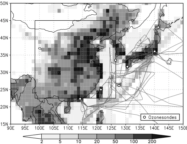
[19] To investigate the impacts of model resolution on
chemical tracers, we first examine boundary layer produc-tion of O3 in springtime over continental east Asia (22 –
45N, 98 – 126E). Figure 3 highlights the location of the main precursor sources over this region at the highest model resolution used in these studies (T106). It also shows the ozonesonde launch sites and aircraft flight tracks from the TRACE-P campaign in spring 2001, and these measurement data provide a valuable standard against which the CTM results can be tested. The mean net production below 750 hPa in March and April 2001 is shown in Figure 4 at four different model resolutions using the same precursor emissions. In the standard model configuration, there is a 7% reduction in net regional production between T21 (5.6) and T106 (1.1) resolution. The 10% decrease in gross production is partly offset by a decrease in destruction. This change is controlled principally by the effects of reduced horizontal averaging on chemical production and by aver-aging of the horizontal and vertical transport fluxes into and out of the region, and is similar in magnitude to that seen in previous studies [e.g.,Kentarchos et al., 2001;Esler et al., 2004;Wild et al., 2004].
[20] At higher resolutions as the spatial scales approach
those critical for O3 production, the simulated production
This convergence will not include the effects of plume processes operating at small scales, which are not included in the model, but should capture the larger-scale processing appropriate to the 50-km scale of precursor emissions used here. Figure 4 shows that there is a slow convergence with resolution that is almost linear with the horizontal grid resolution. This suggests errors in net production of about 4% at T42 and almost 9% at T21. However, even at T106 the spatial scales remain larger than are required for appropriate simulation of regional O3 production, and
production is still overestimated by about 2%. A key question is what additional error due to even higher reso-lution structures would appear when we include the small-scale processing associated with urban plumes. Modeling studies of urban airsheds and polluted continental regions indicate that spatial scales of less than 20 km may be
required to accurately model O3 production [Sillman et
al., 1990;Jang et al., 1995a].
[21] The two alternative model formulations, (1) using a
1-hour mixed boundary layer and (2) including the effects of aerosol on photolysis rates, are also shown in Figure 4. These formulations demonstrate the robustness of the results for altered horizontal resolution, and allow the errors due to resolution to be compared with those due to other model treatments. More efficient boundary layer mixing gives 5% greater net regional production than the standard case because of the more rapid distribution of surface emissions through the boundary layer. Inclusion of aerosols gives a 10% reduction in net regional production, as sunlight in the boundary layer is attenuated and O3 production is
conse-quently reduced. However, the convergence of the regional net O3production with increasing resolution is the same for
[image:5.612.153.457.58.495.2]these two cases as for the standard model formulation.
Figure 1. (a) Surface CO2 abundances (ppm) averaged over year 10 of fossil fuel emissions (1995
pattern, 2.92 ppm/yr) with zero initialization. (b) Difference in surface CO2abundances (ppm), doubled
Figure 2. Convergence factors, k, for the 1 – 2 – 4 and 2 – 4 – 8 sequences of doubled resolution CTM runs (initialized 1 July and run with fossil fuel CO2until 14 September).kfactors are calculated from
instantaneous surface CO2 abundances, f, as (f4f2)/(f2f1) and (f8f4)/(f4f2) respectively, and are
plotted only where the first correction of the sequence,f2f1orf4f2, exceeds 0.04 ppm.
Figure 3. Surface NOxemissions (inmg m 2
[image:6.612.155.454.452.682.2][22] To what extent does increased model resolution
affect the simulation of observations in or downwind of the region? Figure 5 shows a comparison with O3 in the
boundary layer (below 800 hPa) at the seven sonde launch sites over the western Pacific shown in Figure 3 and at two additional locations at Hilo, Hawaii, and Trinidad Head, California. These include launch sites close to major source regions and at remote locations and thus provide a good test of a range of dilution and mixing conditions for O3.
Comparison statistics for the 137 sonde profiles available between February and April 2001 are shown for each CTM resolution in Table 1. Increased resolution typically leads to small increases in correlation coefficient,r, slopes closer to unity, and reduction in the mean and absolute bias, and thus to improvements by all measures. While this is encouraging, it should be noted that these improvements are not statisti-cally significant at a 90% level (applying Student’s t-test). Differences between the model and the measurements are dominated by other errors (in transport, emissions, chemical mechanism and simulation of dynamical features such as
plume lofting and boundary layer mixing depth) rather than by chemical nonlinearity on these scales. Systematic differ-ences by location are revealed more clearly by comparing the T21 and T106 simulations shown in Figure 5. At Cheju Island, Korea (pluses), a relatively clean location sampling outflow from China, the mean bias is reduced from 6.9 to 1.5 ppb and the absolute bias from 12 to 4 ppb. Over Taiwan (triangles), the mean bias is reduced from 3.6 to
0.1, but the absolute bias is only reduced from 14 to 12 ppb, highlighting the sensitivity of this site to local sources. The sonde locations over Japan show modest improve-ments, but boundary layer O3is still overestimated at these
sites by an average of 14 ppb, suggesting that in addition to resolution issues there may be problems in the CTM with sources or sinks at higher latitudes. Despite the clear overall improvement at T106, in individual cases the comparison may be poorer than at T21, reflecting sampling issues and sensitivity to the location of meteorological features.
[23] Previous studies comparing FRSGC/UCI CTM
[image:7.612.155.457.52.254.2]sim-ulations with TRACE-P aircraft measurements made during
Figure 4. Boundary layer O3production (surface to 750 hPa) over east Asia in March/April 2001.
Figure 5. Mean boundary layer O3below 800 hPa from the FRSGC/UCI CTM against that from 137
[image:7.612.96.515.533.703.2]spring 2001 demonstrated that the geographical patterns of O3production were captured well, but noted a number of
biases including overestimation of lower-tropospheric O3
and underestimation of NOx and O3 production in the
midtroposphere over the western Pacific [Wild et al., 2004]. Coarse resolution leading to excessive O3production
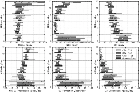
[image:8.612.60.300.107.161.2]in source regions and reduced precursor export were spec-ulated as one cause of these biases. To test this, we show the impact of resolution on the simulation of measurements made along the DC-8 and P-3B aircraft flight tracks in Figure 6. At most altitudes there is a consistent improve-ment in simulation of the statistical distributions of O3, NOx
and CO measurements. However, significant discrepancies clearly remain, particularly for NOx in the midtroposphere
between 4 and 8 km, where the impacts of resolution appear small. The underestimation here may reflect omission of the impacts of heterogeneous chemistry on aerosol which may increase the ratio of NOxto NOyover the western Pacific in
spring [Phadnis and Carmichael, 2000]. Although the means and medians both improve with resolution, the observed NOx and CO distributions are strongly skewed,
with large differences between mean and median values and much higher 90th percentile abundances than modeled. Our inability to capture this behavior is as expected since we still cannot resolve pollution plumes at resolutions below 120 km.
[24] In Figure 6 we also compare CTM-calculated
chem-ical tendencies for O3along the aircraft flight tracks with
those calculated using the Georgia Tech/NASA Langley photochemical steady state box model [Crawford et al., 1999] constrained by 1-min averaged precursor measure-ments (a spatial scale of about 14 km). Both formation and destruction terms closely match the in situ calculations at T106 resolution (120 km). However, underestimation of NOx levels at T106 leads to continued underestimation of
O3formation in the free troposphere in the CTM.
[25] The alternative model formulations have little effect
on these comparisons with observations. Inclusion of aero-sol leads to marginal improvements in the mean and absolute biases in boundary layer O3 at all ozonesonde
Table 1. Correlation Coefficient (r), Slope of Linear Regression and Mean and Absolute Biases Between Boundary Layer O3 Below 800 hPa on Ozonesondes and in the FRSGC/UCI CTM for 9 Locations Around the North Pacific, February to April 2001a
r Slope Mean Bias Absolute Bias
T21 0.526 1.17 7.05 12.03
T42 0.567 1.11 7.15 11.20
T63 0.574 1.04 6.41 10.52
T106 0.578 1.01 5.95 9.87
a
[image:8.612.65.545.366.680.2]Biases are in ppb.
locations, but has very little effect on the flight track comparisons. Differences with the bulk-mixed boundary layer treatment are negligible.
5. Global Changes
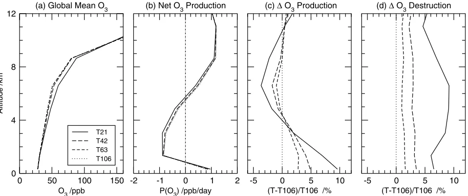
[26] The global tropospheric O3burden (Tg) and budget
terms (Gg/day) averaged over March and April 2001 are given in Table 2 for the standard scenario, and the profiles of these terms are shown in Figure 7. The mean tropospheric O3burden is 3% less at T106 than at T42, reflecting a 2%
reduction in gross production together with an increase in deposition and a reduction in input from the stratosphere. The global gross O3destruction scales with the burden, and
the lifetimes defined from destruction are nearly constant from T21 to T106. The tracer tropopause is defined dynam-ically here using the 120 ppb isopleth of the Linoz tracer [McLinden et al., 2000], and influx from the stratosphere decreases dramatically (12%) from T21 to T42, but little from T42 to T106. It is likely that the sharply defined midlatitude tropopause jet structures in O3, common at this
time of year [see Wild et al., 2003], are not resolved horizontally at T21 and thus are incorrectly mixed into the troposphere. Evidence for this is seen in Figure 7 where the O3abundances at T21 are anomalously high in the middle
and upper troposphere relative to the other resolutions.
Interestingly, surface deposition, which is comparable to the stratospheric source, becomes a more effective sink for O3 as resolution increases even though surface O3 levels
change little. This reflects changes in geographic distribu-tion, with higher O3abundances, reduced chemical
destruc-tion and greater deposidestruc-tion in remote continental regions away from major emission sources. The chemical lifetime of CH4against OH destruction is 3% longer at T106 than
T42, mirroring the 3% decrease in O3burden, and suggests
a reduced abundance of OH radicals and thus slower oxidation of other hydrogenated trace gases.
[27] The altitude profile of net O3production (Figure 7b)
is similar across all resolutions: net production is positive below 1 km altitude, net loss occurs from 1 to 6 km, and net production is positive again above 6 km. Gross production (Figure 7c) shows the uniform impact of increasing resolu-tion from T21 to T106. Below 4 km, gross producresolu-tion decreases with resolution, and from 4 to 10 km, it increases. At lower resolution, gross O3 production is higher in the
boundary layer because of the failure to resolve pollution plumes. In the midtroposphere, gross production is less, reflecting either lower levels of NOx, CO and hydrocarbons
exported from surface source regions or more efficient oxidation of NOx to NOz due to higher O3. In the upper
troposphere O3 production is marginally higher than at
[image:9.612.107.509.75.162.2]T106 because of greater deep-convective lofting of NOx.
Table 2. Global Oxidant Budgets for March/April 2001
T21 T42 T63 T106
Mean O3burden, Tg 294 284 278 275
Gross production, Gg/day 12,290 12,130 12,040 11,880
Gross destruction, Gg/day 12,120 11,650 11,450 11,290
Net O3production, Gg/day 169 480 594 583
O3deposition, Gg/day 2,090 2,210 2,250 2,300
O3stratosphere/troposphere exchange, Gg/day 2,000 1,760 1,670 1,730
O3chemical lifetime,adays 24.25 24.34 24.25 24.34
CH4lifetime versus OH, years 8.06 8.32 8.44 8.57
a
Lifetime defined as burden divided by gross destruction.
Figure 7. Impacts of resolution on the global O3budget for March/April 2001 showing (a) the mean O3
[image:9.612.69.548.501.702.2]In contrast, gross destruction shows no altitude patterns and decreases uniformly with resolution in response to the reduced O3burden (Figure 7d).
6. Response to Regional Emissions
[28] The regional and global changes in O3attributable to
emissions from east Asia are assessed by applying a 10% perturbation to industrial emissions of NOx, CO and NMHC
over continental east Asia (see Figure 3) for a 5-day period from 2 to 6 March 2001 and then following the buildup and decay of O3from this pulse for the following 6 weeks. The
day-to-day variation in O3production over the region due to
meteorological factors in springtime is about 15% (1s) [Wild et al., 2004], and the perturbation is therefore applied for a 5-day period to reduce the bias introduced by the pattern of meteorological systems present on any single day. [29] The additional O3production following this pulse is
shown in Figure 8 at T21 and T106 resolution. About 85% of additional production within the boundary layer over east Asia occurs during the first 5 days, but production continues in the free troposphere for several weeks. We find that 80% of global production occurs in the first three weeks and 90% occurs during the 6-week period analyzed here.
[30] The transport and evolution of the plume is illustrated
in Figure 9 which shows the additional net O3production
integrated over the 6-week period. To highlight the location of production, the additional mass of O3produced over the
period is averaged over the appropriate column or meridi-onal volume and is expressed in ppb in Figure 9. Production is greatest in the boundary layer over the emission region, but considerable additional production occurs in a low-level plume centered at about 3 km altitude extending across the Pacific. The effects of deep convective lifting are seen in a separate region of production about 10 km above the emission region. Recirculation of air around a high-pressure region over the eastern Pacific leads to slower eastward transport and subsidence, and the longer residence times and thermal degradation of peroxyacetyl nitrate (PAN) lead to greater cumulative O3production in this region, as found
in previous studies [Kotchenruther et al., 2001;Heald et al.,
2003; Wild et al., 2003; Hudman et al., 2004]. Increased destruction of O3is seen in the marine boundary layer and
in outflow north and south of the emission region where additional loss of the excess O3 is greater than formation
from the exported precursors.
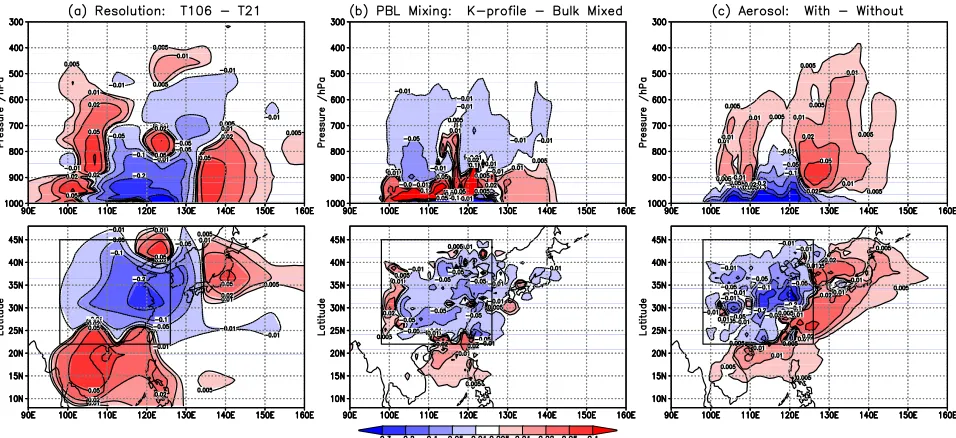
[31] The impacts of model resolution on the location of
O3production are shown in Figure 10. Increasing the model
resolution from T21 to T106 leads to a reduction in the integrated net production over the region (from 58.8 to 45.5 Gg) with the largest reductions below 900 hPa over eastern China, where emissions are highest. Downwind over the western Pacific net production at T106 is reduced in the midtroposphere but is enhanced in the lower troposphere where the boundary layer export of NOxis larger and that of
[image:10.612.156.455.57.242.2]O3is smaller. The net loss over southeast Asia is smaller at
Figure 8. Cumulative additional O3production in the east Asian boundary layer (below 750 hPa) and in
the global troposphere following a 5-day pulse of O3precursors over east Asia in March 2001.
Figure 9. Cumulative net O3production (in ppb) over a
6-week period caused by a 5-day pulse of O3precursors over
east Asia in March 2001 showing the (top) vertical extent (meridionally averaged between 6 and 50N) and (bottom) horizontal extent (column-averaged) of O3 production at
[image:10.612.314.551.472.659.2]T106 than at T21 because of lower O3abundance over east
Asia, a longer NOxlifetime, and greater net transport out of
the region. The change in O3 production with resolution
outside east Asia is small and hence the reduction in the global burden is dominated by changes in gross production over the emission region itself (15.5 Gg out of a total of 19.1 Gg).
[32] The impact of bulk mixing of the boundary layer
every hour is shown in Figure 10b. Using the standard K-profile scheme for boundary layer turbulence rather than a 1-hour mixing leads to a reduction in regional net produc-tion from 48.2 to 45.5 Gg at T106. The less efficient vertical mixing is analogous to the reduced horizontal mixing associated with higher resolution. Production is increased in the lower boundary layer where precursor levels are higher, but it is reduced in the upper layers where precursors are lower and at the surface over high-emission regions where direct removal of O3 by reaction with NOx is
important, see Figure 10b. Larger NOxexport to the marine
boundary layer is balanced by reduced export at higher altitudes, and the net impact on gross global production is a reduction of only 2%, from 215 to 212 Gg.
[33] The impact of including aerosols in the
photochem-istry is shown in Figure 10c. O3production is reduced in the
boundary layer because of the attenuation of sunlight but is increased at higher altitudes by scattering and by increased levels of unreacted precursors escaping the boundary layer. The effect on regional net O3 production is a reduction of
16% (from 45.5 to 38.1 Gg at T106), but 10% higher export of NOxleads to greater O3production immediately
down-wind of the region in outflow over the western Pacific, and the net impact on the gross global production is a reduction of only 3%, from 212 to 206 Gg. In this case the shift in the timescale to produce O3is clear, as production is relocated
from inside the region to outside it, and the time taken to reach 50% of the global production extends from 3.3 days to 4.0 days.
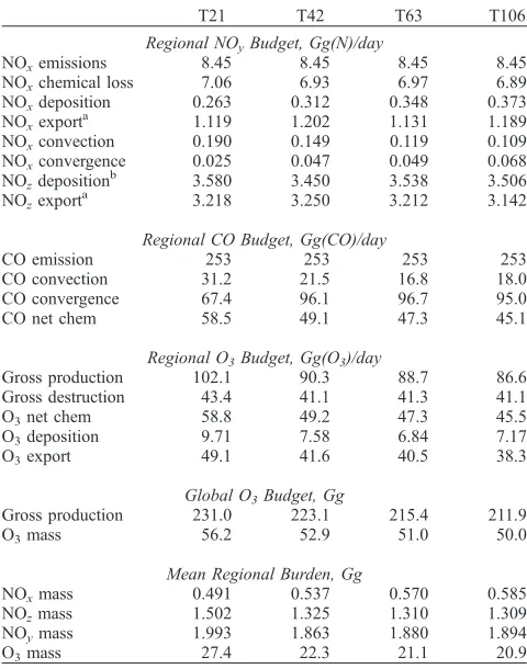
[34] The changes in the budget terms of O3, CO and NOy
due to the 5-day emission pulse are shown in Table 3. The differences are integrated over the 6-week simulation period and are then renormalized by dividing by 5 days and by the 10% emissions scale factor applied. The resulting budget terms in Table 3 then represent the daily impact of total east Asian industrial emissions, are effectively independent of the period and scale factor used, and can be compared directly with the budget terms in Table 2. More than 80% of the NOx released is oxidized to HNO3and PAN (together
denoted here as NOz) over the region, 3 – 4% is deposited,
and the remainder is transported out of the region, mostly horizontally within the boundary layer. At higher resolution, the reduced averaging and greater separation of polluted and clean regions leads to slower removal of NOx. The chemical
lifetime of NOxis 22% longer at T106 than at T21, but the
total chemical loss is almost unchanged, and thus the regional burden is correspondingly greater (by 27%). Net O3production is almost 25% less at T106 than at T21, and
the regional burden, deposition and export of O3 are
affected by a similar amount. Slower oxidation of NOx to
HNO3 and PAN leads to a lower abundance of these
species, and to greater direct export of NOx relative to
NOz at T106, but the total export of NOy is almost
unchanged. Gross O3 production outside the emission
region shows only small differences.
7. Errors and Convergence in the Ozone Budget
[35] The progression from T21 to T106 resolution shows
a generally consistent decline in O3 budget terms and
[image:11.612.68.546.57.276.2]burdens (Tables 2 and 3), with the largest reduction in error
Figure 10. Differences in the cumulative net O3production (in ppb) following a 5-day pulse of O3
on moving from T21 to T42, and with smaller differences between T63 and T106. We derive values for the limit of infinite resolution, T1, on the basis of convergence of the sequence T42 – T63 – T106, and use the difference between values at T1and those at a given resolution to represent the error,e, at that resolution, e.g.,e106= T106-T1, as shown
in Table 4. We look for a Richardson-like extrapolation to derive T1, assuming that the absolute error in a given calculation is proportional to some power of the grid sizeh,
e/hN, where h is 1.1for T106, 1.9for T63, 2.8for T42, and 5.6for T21. The O3production terms and burdens are
well behaved, with N 2, corresponding to a numerical solution that is second-order accurate (e.g., trapezoidal integration). For some quantities, such as the net strato-spheric influx or the chemical lifetime of O3, the sequence is
not monotonic. In these cases the changes across resolutions are usually small and hence so are the errors.
[36] On a global scale, the errors in global tropospheric
O3 burden at T42 are about 10 Tg (4%), while the gross
production is overestimated by about 420 Gg/day (4%, 150 Tg/yr). In terms of attributing the impact of east Asian emissions, we find that at T42 the error in the net regional production over east Asia is 6.2 Gg/day (14%), and that the corresponding error in global O3burden is 3.4 Gg (7%). At
T106 these errors are smaller but still significant, 2.5 Gg/ day (6%) and 0.48 Gg (1%), respectively. The impacts on the global OH budget are also significant, and OH is
overestimated at all resolutions. The lifetime of CH4 to
oxidation by OH, about 8.7 years, is underestimated by 0.4 years (5%) at T42, and is still underestimated by 0.2 years (2%) at T106.
[37] Altering the horizontal resolution leads to changes in
the relative importance of different transport mechanisms. Averaging advective fluxes over adjacent grid boxes when transforming to lower resolution smoothes out the high-frequency variability of the met fields and thus leads to slower transport where strong tracer gradients are present. This averaging is particularly important for vertical trans-port [Wang et al., 2004] where we find that vertical advection of CO, driven by convergence and cyclonic lifting, is 30% less over east Asia at T21 than at T106. In contrast, convective lifting is 70% greater at T21 than at T106 for both CO and NOx. For short-lived O3precursors
such as NOx and isoprene, convection is the dominant
export mechanism, and thus resolution-related errors in convection may have significant implications for O3
pro-duction in the free troposphere, where the lifetimes of both NOx and O3 are longer. Overestimation of the convective
export of short-lived species at coarse resolution has also been noted in previous modeling studies [Jang et al., 1995a;
Krol et al., 2005]. Over east Asia in spring, convection is dominated by shallow convective processes in clouds asso-ciated with frontal systems, whereas much of the outflow of pollution from east Asia occurs at low altitudes behind cold fronts [Carmichael et al., 1998]. This separation between regions of convection and elevated pollution is minimized by averaging meteorological variables and demonstrates that high-resolution models are necessary to simulate the transport of ozone and precursors associated with midlati-tude cyclones.
8. Conclusions
[38] We have used a global CTM at a sequence of four
horizontal resolutions between T21 (5.6) and T106 (1.1) in spring 2001 to determine the errors in simulating tropo-spheric O3 due to horizontal resolution. Agreement with
atmospheric measurements is consistently better at higher resolution as seen from tracer correlations, slopes and biases in O3 and precursor abundances between the CTM and
[image:12.612.60.300.86.391.2]TRACE-P aircraft and ozonesonde observations. The biases are not improved at a statistically significant level, however, Table 3. Changes in the Budgets of NOy, CO and O3 Due to
Industrial Emissions Over East Asia in March 2001
T21 T42 T63 T106
Regional NOyBudget, Gg(N)/day
NOxemissions 8.45 8.45 8.45 8.45
NOxchemical loss 7.06 6.93 6.97 6.89
NOxdeposition 0.263 0.312 0.348 0.373
NOxexporta 1.119 1.202 1.131 1.189
NOxconvection 0.190 0.149 0.119 0.109
NOxconvergence 0.025 0.047 0.049 0.068
NOzdeposition b
3.580 3.450 3.538 3.506 NOzexporta 3.218 3.250 3.212 3.142
Regional CO Budget, Gg(CO)/day
CO emission 253 253 253 253
CO convection 31.2 21.5 16.8 18.0 CO convergence 67.4 96.1 96.7 95.0
CO net chem 58.5 49.1 47.3 45.1
Regional O3Budget, Gg(O3)/day
Gross production 102.1 90.3 88.7 86.6 Gross destruction 43.4 41.1 41.3 41.1 O3net chem 58.8 49.2 47.3 45.5 O3deposition 9.71 7.58 6.84 7.17
O3export 49.1 41.6 40.5 38.3
Global O3Budget, Gg
Gross production 231.0 223.1 215.4 211.9
O3mass 56.2 52.9 51.0 50.0
Mean Regional Burden, Gg
NOxmass 0.491 0.537 0.570 0.585
NOzmass 1.502 1.325 1.310 1.309
NOymass 1.993 1.863 1.880 1.894
O3mass 27.4 22.3 21.1 20.9
aTotal tendency due to horizontal, convergent and convective transport mechanisms.
bNO
zdefined as all NOyspecies except NOx.
Table 4. Convergence and Resolution Errors in Oxidant Budgetsa
T1b
Nc e21d e42 e63 e106
Global Budgets (From Table 2)
Global gross P(O3) 11,710 1.0 578 422 335 169 Global O3burden, Tg 273.6 2.2 20.2 10.0 4.1 1.3 CH4lifetime, years 8.73 1.0 0.67 0.41 0.29 0.16
Impacts of East Asian Emissions (From Table 3)
Regional net P(O3) 43.0 1.0 15.8 6.2 4.3 2.5 Regional gross P(O3) 84.1 1.8 18.0 6.2 4.5 2.5 Regional O3burden 20.8 2.9 6.6 1.4 0.3 0.1 Global gross P(O3) 210.4 2.3 20.6 12.8 5.0 1.5 Global O3burden 49.6 2.1 6.6 3.4 1.4 0.5
aBudgets in Gg/day and burdens in Gg unless stated. b
Corrected budget based on T42 – T63 – T106 convergence. cOrder N used in Richardson Extrapolation.
d
[image:12.612.311.553.589.707.2]indicating that differences between the model and measure-ments are still dominated by other sources of error, e.g., emissions, chemical mechanism, transport, and dynamical features such as plume lofting and convection.
[39] Increased resolution leads to reduced O3production
over polluted regions, lower OH radical concentrations and slower removal of precursors such as NOx and CO. The
export of these precursors from east Asia is higher, but subsequent O3 production in the free troposphere is not
greatly affected. One reason is that the importance of convection is exaggerated at coarse resolution, enhancing the export of NOxto the mid- and upper troposphere where
O3production is more efficient, and countering the effect of
dilution of emissions over the larger grid boxes that increases both O3production and oxidation of NOx. Influx
of O3from the stratosphere is greatly overestimated at T21,
but is basically unchanged over the T42 – T63 – T106 se-quence. The chemical lifetime of tropospheric O3, defined
as the global burden divided by gross destruction, is nearly constant across all resolutions. Overestimation of O3
pro-duction and greater removal of greenhouse gases such as CH4 at low resolution will lead to biases in
climate-chemistry studies that may be counteracting, like those seen by previous studies [Mayer et al., 2000;Wild and Prather, 2000]. Excessive O3production in polluted regions is also
likely to have implications for source-attribution studies of tropospheric O3, which may be biased toward nearby
regions because of the shorter timescales for production. [40] In a simplified case study of transport of a passive
tracer, we have demonstrated that the errors in a sequence of resolutions converges geometrically. Applying this ap-proach to the full chemistry CTM we show that O3
production is consistently overestimated in coarse-resolu-tion models and that in most cases the O3budget and CH4
lifetime show a converging sequence with improved reso-lution. A case study with enhanced emissions over east Asia allows us to derive errors in additional net O3production
over the region of 27% at T21, 13% at T42, 9% at T63 and 5% at T106. In this study the resolution errors are based on the use of emissions averaged over 50 km scales, and therefore the convergence with resolution does not include the effects of highly concentrated urban and industrial pollution plumes.
[41] Comparing alternative CTM formulations, we find
that instantaneous vertical mixing of the boundary layer has a similar impact to coarse horizontal resolution, increasing O3production in polluted regions but decreasing it outside.
The effects of a realistic aerosol distribution on photolysis rates leads to reduced O3production over polluted regions
but has little global impact because more precursors are exported and production shifts to the global troposphere. Thus increased resolution, improved treatment of boundary layer mixing, and inclusion of the impacts of aerosol on photolysis all lead to reductions in local O3production and
a reduced tropospheric O3burden. Coarse-resolution
mod-els of O3chemistry without aerosols may overestimate O3
production by more than 20% and thus many early model studies such as those summarized by Prather and Ehhalt
[2001] may be affected by this bias. However, there are certainly other sources of errors in these models, such as the oversimplification of hydrocarbon chemistry, that might provide a countering bias.
[42] Acknowledgments. The authors are grateful to Jostein Sundet (University of Oslo) for generating and supplying the ECMWF-IFS forecast data under Special Project SPNOO3CL at the ECMWF.
References
Allen, D. J., and K. E. Pickering (2002), Evaluation of lightning flash rate parameterizations for use in a global chemical transport model,J. Geo-phys. Res.,107(D23), 4711, doi:10.1029/2002JD002066.
Berntsen, T., I. S. A. Isaksen, W. C. Wang, and X. Z. Liang (1996), Impacts of increased anthropogenic emissions in Asia on tropospheric ozone and climate,Tellus, Ser. B,48, 13 – 32.
Bian, H., M. J. Prather, and T. Takemura (2003), Tropospheric aerosol impacts on trace gas budgets through photolysis, J. Geophys. Res.,
108(D8), 4242, doi:10.1029/2002JD002743.
Brenkert, A.L. (1998), Carbon dioxide emission estimates from fossil-fuel burning, hydraulic cement production, and gas flaring for 1995 on a one degree grid cell basis, http://cdiac.esd.ornl.gov/ndps/ndp058a.html, Car-bon Dioxide Inf. Anal. Cent., Oak Ridge Natl. Lab., Oak Ridge, Tenn. Carmichael, G., I. Uno, M. Phadnis, Y. Zhang, and Y. Sunwoo (1998),
Tropospheric ozone production and transport in the springtime in east Asia,J. Geophys. Res.,103, 10,649 – 10,672.
Chameides, W. L., and J. C. G. Walker (1973), A photochemical theory of tropospheric ozone,J. Geophys. Res.,78, 8751 – 8760.
Chatfield, R. B., and A. C. Delany (1990), Convection links biomass burn-ing to increased tropical ozone: However, models will tend to overpredict O3,J. Geophys. Res.,95, 18,473 – 18,488.
Crawford, J., et al. (1999), Assessment of upper tropospheric HOxsources
over the tropical Pacific based on NASA GTE/PEM data: Net effect on HOx and other photochemical parameters, J. Geophys. Res., 104,
16,255 – 16,274.
Crutzen, P. J. (1974), Photochemical reactions initiated by and influencing ozone in unpolluted tropospheric air,Tellus,26, 47 – 57.
Douglass, A. R., M. J. Prather, T. M. Hall, S. E. Strahan, P. J. Rasch, L. C. Sparling, L. Coy, and J. M. Rodriguez (1999), Choosing meteorological input for the global modeling initiative assessment of high-speed aircraft,
J. Geophys. Res.,104, 27,545 – 27,564.
Duce, R. A., C. K. Unni, B. J. Ray, J. M. Prospero, and J. T. Merrill (1980), Long-range atmospheric transport of soil dust from Asia to the tropical North Pacific: Temporal variability,Science,209, 1522 – 1524. Esler, J. G., G. J. Roelofs, M. O. Ko¨hler, and F. M. O’Connor (2004), A
quantitative analysis of grid-related systematic errors in oxidising capa-city and ozone production rates in chemistry transport models,Atmos. Chem. Phys.,4, 1781 – 1795.
Gurney, K. R., et al. (2003), TransCom3 CO2inversion intercomparison: 1. Annual mean control results and sensitivity to transport and prior flux information,Tellus, Ser. B,55, 555 – 579.
Hauglustaine, D. A., F. Hourdin, L. Jourdain, M.-A. Filiberti, S. Walters, J.-F. Lamarque, and E. A. Holland (2004), Interactive chemistry in the Laboratoire de Me´te´orologie Dynamique general circulation model: Description and background tropospheric chemistry evaluation,J. Geo-phys. Res.,109, D04314, doi:10.1029/2003JD003957.
Heald, C. L., et al. (2003), Asian outflow and trans-Pacific transport of carbon monoxide and ozone pollution: An integrated satellite, aircraft and model perspective, J. Geophys. Res., 108(D24), 4804, doi:10.1029/ 2003JD003507.
Holtslag, A. A. M., and B. A. Boville (1993), Local versus nonlocal bound-ary layer diffusion in a global climate model,J. Clim.,6, 1825 – 1842. Horowitz, L. W., et al. (2003), A global simulation of tropospheric ozone
and related tracers: Description and evaluation of MOZART, version 2,
J. Geophys. Res.,108(D24), 4784, doi:10.1029/2002JD002853. Hourdin, F., and A. Armengaud (1999), The use of finite-volume methods
for atmospheric advection of trace species. Part 1: Test of various for-mulations in a general circulation model,Mon. Weather Rev.,127, 822 – 837.
Houweling, S., F. Dentener, and J. Lelieveld (1998), The impact of non-methane hydrocarbon compounds on tropospheric photochemistry, J. Geophys. Res.,103, 10,673 – 10,696.
Hsu, C. J., M. J. Prather, O. Wild, J. K. Sundet, I. S. A. Isaksen, E. V. Browell, M. A. Avery, and G. W. Sachse (2004), Are the TRACE-P measurements representative of the western Pacific during March 2001?,J. Geophys. Res.,109, D02314, doi:10.1029/2003JD004002. Hudman, R. C., et al. (2004), Ozone production in transpacific Asian
pollu-tion plumes and implicapollu-tions for ozone air quality in California,J. Geo-phys. Res.,109, D23S10, doi:10.1029/2004JD004974.
Jacob, D. J. (2000), Heterogeneous chemistry and tropospheric ozone, At-mos. Environ.,34, 2131 – 2159.
Jacob, D. J., et al. (2003), Transport and Chemical Evolution over the Pacific (TRACE-P) aircraft mission: Design, execution and first results,
J. Geophys. Res.,108(D20), 9000, doi:10.1029/2002JD003276. Jaffe, D., et al. (1999), Transport of Asian air pollution to North America,
Geophys. Res. Lett.,26, 711 – 714.
Jang, J. C., H. E. Jeffries, D. W. Byun, and J. E. Pleim (1995a), Sensitivity of ozone to model grid resolution: Part 1. Application of high-resolution regional acid deposition model,Atmos. Environ.,29, 3085 – 3100. Jang, J. C., H. E. Jeffries, and S. Tonnesen (1995b), Sensitivity of ozone to
model grid resolution: Part 2. Detailed process analysis for ozone chem-istry,Atmos. Environ.,29, 3101 – 3114.
Kentarchos, A. S., G. J. Roelofs, and J. Lelieveld (2001), Altitude distribu-tion of tropospheric ozone over the Northern Hemisphere during 1996, simulated with a chemistry-general circulation model at two different horizontal resolutions,J. Geophys. Res.,106, 17,453 – 17,469. Kiley, C. M., et al. (2003), An intercomparison and evaluation of
aircraft-derived and simulated CO from seven chemical transport models during the TRACE-P experiment, J. Geophys. Res., 108(D21), 8819, doi:10.1029/2002JD003089.
Kinnison, D. E., et al. (2001), The Global Modeling Initiative assessment model: Application to high-speed civil transport perturbation,J. Geophys. Res.,106, 1693 – 1711.
Kotchenruther, R. A., D. A. Jaffe, and L. Jaegle (2001), Ozone photochem-istry and the role of PAN in the springtime northeastern Pacific tropo-sphere: Results from the PHOBEA campaign,J. Geophys. Res.,106, 28,731 – 28,741.
Krol, M., S. Houweling, B. Bregman, M. van den Broek, A. Segers, P. van Velthoven, W. Peters, F. Dentener, and P. Bergamaschi (2005), The two-way nested chemistry-transport zoom model TM5: Algorithm and appli-cations,Atmos. Chem. Phys.,5, 417 – 432.
Lin, X., M. Trainer, and S. C. Liu (1988), On the nonlinearity of the tropospheric ozone production,J. Geophys. Res.,93, 15,879 – 15,888. Liu, S. C., M. Trainer, F. C. Fehsenfeld, D. D. Parrish, E. J. Williams, D. W.
Fahey, G. Hu¨bler, and P. C. Murphy (1987), Ozone production in the rural troposphere and the implications for regional and global ozone distributions,J. Geophys. Res.,92, 4191 – 4207.
Martin, R. V., D. J. Jacob, R. M. Yantosca, M. Chin, and P. Ginoux (2003), Global and regional decreases in tropospheric oxidants from photoche-mical effects of aerosols,J. Geophys. Res.,108(D3), 4097, doi:10.1029/ 2002JD002622.
Mayer, M., C. Wang, M. Webster, and R. G. Prinn (2000), Linking local air pollution to global chemistry and climate,J. Geophys. Res., 105, 22,869 – 22,896.
McLinden, C. A., S. Olsen, B. Hannegan, O. Wild, M. J. Prather, and J. Sundet (2000), Stratospheric ozone in 3-D models: A simple chemistry and the cross-tropopause flux,J. Geophys. Res.,105, 14,653 – 14,665. Park, R. J., K. E. Pickering, D. J. Allen, G. L. Stenchikov, and M. S.
Fox-Rabinovitz (2004), Global simulation of tropospheric ozone using the University of Maryland Chemical Transport Model (UMD-CTM): 2. Regional transport and chemistry over the central United States using a stretched grid,J. Geophys. Res., 109, D09303, doi:10.1029/ 2003JD004269.
Phadnis, M. J., and G. R. Carmichael (2000), Numerical investigation of the influence of mineral dust on the tropospheric chemistry of east Asia,
J. Atmos. Chem.,36, 285 – 323.
Pickering, K. E., Y. Wang, W.-K. Tao, C. Price, and J.-F. Mu¨ller (1998), Vertical distributions of lightning NOx for use in regional and global
chemical transport models,J. Geophys. Res.,103(D23), 31,203 – 31,216. Prather, M. J. (1986), Numerical advection by conservation of second-order
moments,J. Geophys. Res.,91, 6671 – 6681.
Prather, M., and D. Ehhalt (2001), Atmospheric chemistry and greenhouse gases, inClimate Change 2001: The Scientific Basis, pp. 239 – 287, Cam-bridge Univ. Press, New York.
Rind, D., D. Shindell, P. Lonergan, and N. K. Balachandran (1998), Climate change and the middle atmosphere. Part III: The doubled CO2climate revisited,J. Clim.,11, 876 – 894.
Roelofs, G. J., et al. (2003), Intercomparison of tropospheric ozone models: Ozone transport in a complex tropopause folding event,J. Geophys. Res.,
108(D12), 8529, doi:10.1029/2003JD003462.
Rotman, D. A., et al. (2001), The Global Modeling Initiative assessment model: Model description, integration and testing of the transport shell,
J. Geophys. Res.,106, 1669 – 1691.
Sillman, S., J. A. Logan, and S. C. Wofsy (1990), A regional scale model for ozone in the United States with subgrid representation of urban and power plant plumes,J. Geophys. Res.,95, 5731 – 5748.
Streets, D. G., et al. (2003), An inventory of gaseous and primary aerosol emissions in Asia in the year 2000,J. Geophys. Res.,108(D21), 8809, doi:10.1029/2002JD003093.
Tang, Y., et al. (2003), Impacts of aerosols and cloud on photolysis fre-quencies and photochemistry during TRACE-P: 2. A three-dimensional study using a regional chemical transport model, J. Geophys. Res.,
108(D21), 8822, doi:10.1029/2002JD003100.
Tegen, I., P. Hollrig, M. Chin, I. Fung, D. Jacob, and J. Penner (1997), Contribution of different aerosol species to the global aerosol extinction optical thickness: Estimates from model results,J. Geophys. Res.,102, 23,895 – 23,915.
von Kuhlmann, R., M. G. Lawrence, P. J. Crutzen, and P. J. Rasch (2003), A model for studies of tropospheric ozone and nonmethane hydrocar-bons: Model description and ozone results,J. Geophys. Res.,108(D9), 4294, doi:10.1029/2002JD002893.
Wang, Y. H., D. J. Jacob, and J. A. Logan (1998), Global simulation of tropospheric O3-NOx-hydrocarbon chemistry: 2. Model evaluation and
global ozone budget,J. Geophys. Res.,103, 10,727 – 10,756.
Wang, Y. X., M. B. McElroy, D. J. Jacob, and R. M. Yantosca (2004), A nested grid formulation for chemical transport over Asia: Applications to CO,J. Geophys. Res.,109, D22307, doi:10.1029/2004JD005237. Wesely, M. L. (1989), Parameterization of surface resistances to gaseous
dry deposition in regional-scale numerical models,Atmos. Environ.,23, 1293 – 1304.
Wild, O., and M. J. Prather (2000), Excitation of the primary tropospheric chemical mode in a global 3-D model,J. Geophys. Res.,105, 24,647 – 24,660.
Wild, O., X. Zhu, and M. J. Prather (2000), Fast-J: Accurate simulation of in- and below-cloud photolysis in tropospheric chemical models,J. At-mos. Chem.,37, 245 – 282.
Wild, O., J. K. Sundet, M. J. Prather, I. S. A. Isaksen, H. Akimoto, E. V. Browell, and S. J. Oltmans (2003), CTM Ozone Simulations for spring 2001 over the western Pacific: Comparisons with TRACE-P lidar, ozo-nesondes and TOMS columns, J. Geophys. Res., 108(D21), 8826, doi:10.1029/2002JD003283.
Wild, O., et al. (2004), CTM ozone simulations for spring 2001 over the western Pacific: Regional ozone production and its global impacts,
J. Geophys. Res.,109, D15S02, doi:10.1029/2003JD004041.
M. J. Prather, Earth System Science, University of California, Irvine, CA 92697-3100, USA.