Simulating the Gene Flow of Genetically Modified Maize in Taiwan

http://dx.doi.org/10.4236/as.2014.55045

How to cite this paper: Kuo, B.-J., et al. (2014) Simulating the Gene Flow of Genetically Modified Maize in Taiwan. Agricul-tural Sciences, 5, 440-453. http://dx.doi.org/10.4236/as.2014.55045

Simulating the Gene Flow of Genetically

Modified Maize in Taiwan

Bo-Jein Kuo

, Shuo-Cheng Nieh

, Guang-Jauh Shieh

, Wen-Shin Lin

2_{Crop Science Division, Taiwan Agricultural Research Institute, Council of Agriculture, Executive Yuan, Taichung,} Taiwan

3_{Department of Plant Industry, National Pingtung University of Science and Technology, Pingtung, Taiwan}

Email: *[email protected]

Received 17 February 2014; revised 22 March 2014; accepted 5 April 2014

Copyright © 2014 by authors and Scientific Research Publishing Inc.

This work is licensed under the Creative Commons Attribution International License (CC BY).

http://creativecommons.org/licenses/by/4.0/

Abstract

A field experiment was conducted in Taiwan to measure the cross-pollination (CP) rate of maize pollen recipients from pollen sources using phenotypic marker and to determine the isolation dis- tance between the 2 maize varieties. A waxy variety (Black Pearl) with purple kernels simulated the genetically modified (GM) pollen donor, and another waxy variety (White Pearl) with white kernels simulated the non-GM recipient. For the first crop, the total area was approximately 1.5 ha with a pollen source and recipient acreage ratio of approximately 1:32. For the second crop, the total area was approximately 1.83 ha with a ratio of approximately 1:17.3. The source fields were surrounded by the recipient fields for 2 crop seasons. The results showed that the rate of CP was <0.05% beyond 15 m upwind and 84.8 m downwind in all crop seasons. The CP rate was below 5% at a distance of 10 m in the downwind direction. A sample with 0.24% CP was recorded at 107.3 m downwind; however, the CP rate was 0% at 68 m upwind. Three empirical models were used, that is, exponential, log/log and log/log, and a simplified Gaussian Plume model, to examine the rela-tionship between the CP rates and the source-field distances. All of the models were appropriate for predicting CP rates, and the Gaussian Plume model performed better compared to the empiri-cal models. The results show that it is possible to control CP from foreign pollen by using an ap-propriate isolation distance.

Keywords

Cross-Pollination, Gaussian Plume Model, Gene Flow Model, Maize, Xenia Effect

1. Introduction

In 2012, the global acreage of commercial planting of genetically modified (GM) crops reached 170 million

hectares. The principal GM crops are soybeans, maize, cotton, and canola. Worldwide acreage of GM maize is over 50 million hectares [1]. Maize (Zea mays L) is a monoecious, diclinous, protandrous, and wind-pollinated plant with abundant pollen. Because of the anemophilous characteristic of maize, the principal source of adven-titious mixing between GM and non-GM maize is the gene flow between neighboring fields [2]-[4]. In the Eu-ropean Union (EU), all countries are asked to develop national coexistence measures to ensure that GM crops are below the legal threshold value of 0.9% for labeling GM maize food and feed [5].

To reduce the adventitious presence from source pollen to recipient fields, extensive research has been con-ducted on maize gene flow [2] [6]-[11]. Most of studies measured the levels of cross-pollination in the recipient field at various distances from the pollen source by detecting the xenia effect on the progeny. Hence, the cross-pollination rate of maize recipients is defined as the percentage of off-types in the progeny. Based on scientific results published on maize gene flow and cross-pollination, a range of isolation distances between 10 and 50 m are recommended to maintain the cross-pollination rate below the tolerance threshold of 0.9%. How-ever, an isolation distance of 50 m is necessary for recipient fields smaller than 1 ha and fields of low depth, es-pecially when in the downwind direction [5].

In the past 2 decades, research on biotechnology has been supported to develop GM organisms in Taiwan. Currently, none of GM crops are produced in Taiwan. All GM foods in the domestic market rely on foreign im-ports, particularly maize and soybeans. In 2010, the United States exported more than US$613 million of maize and US$653 million of soybeans to Taiwan. Taiwan is the fifth largest export market for US maize and soybeans. Approximately half of the total US agricultural, fish, and forest products exported to Taiwan are biotechnology products [12]. In Taiwan, food products composed of GM soybeans and corn containing more than 5% trans-genic material by weight of the finished product must be labeled with the words “Genetically Modified” (GM) or “Containing Genetically Modified” soybeans and corn, respectively. Currently, the total acreage of maize is approximately 18,000 ha, in which approximately two-thirds are planted with forage corn and the rest with grain corn. Recently, to increase food security and promote the use of fallow, increasing maize cultivation has been encouraged.

To date no study has been conducted on maize gene flow and cross-pollination on a field-scale level in Tai-wan. Most agricultural fields in Taiwan are fragmented landscapes and spatially heterogeneous with minimal pollen sources and recipients.

The purposes of this study are to detect the cross-pollination (CP) rates of maize at various distances from source plots to recipient fields and to construct a gene flow model. This information is useful for management strategies of GM crops and provides a basis for discussion on the issues of coexistence between GM and non-GM crops in Taiwan.

2. Materials and Methods

2.1. Field Design

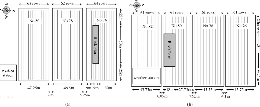
The field experiment was conducted in 2009 at the experimental fields of the Taiwan Agriculture Research In-stitute (TARI), Wufeng, located at 24˚1'N, 120˚41'E. The soil was a silty-clay loam. The total area of the first crop was approximately 1.5 ha with a pollen source and recipient acreage ratio of approximately 1:32. The pol-len source (50 by 9 m) was facing south (Figure 1(a)). Because of irrigation concerns, the experimental fields at TARI were composed of plots with an area of 0.5 ha each. The experimental fields consisted of 3 side-by-side plots (Nos.76, 78, and 80) separated by 2 field roads, 5.25 and 6 m wide, respectively. The total area of the second crop was approximately 1.83 ha with a ratio of approximately 1:17.3. The source plot (50 by 20 m) was located in a northward direction (Figure 1(b)). The experimental fields included 4 plots (Nos. 76, 78, 80, and a portion of No. 82) separated by 3 field roads (4.1, 7.95, and 6.05 m wide, respectively). The source fields for the 2 crop seasons were surrounded by the recipient fields.

2.2. Plant Materials and Planting Dates

47.25m 46.5m 9m 9m 9m 30m

6m 5.25m

weather station

25

m

50

m

25

m

63 rows 62 rows 64 rows

No.80 No.78 No.76

W

S

E

N

B

lack

P

ear

l

6.05m 7.95m

weather station

25

m

50

m

25

m

61 rows

No.80 No.78 No.76

W

S

E

N

B

lack

P

ear

l

61 rows 61 rows 61 rows

4.1m 45.75m 18m 27.75m 45.75m 45.75m

No.82

(a) (b)

Figure 1. Field design of the experiments in 2009. (a) The first crop season; (b) The second crop season. The gray area is for pollen source and the remainder area is for recipient.

Table 1. Planting material, dimensions, sowing date, tasseling date and silking date.

Crop

season Dimensions

Size of

source plot Hybrid name

Date

Planting 50% pollen shed 50% silking

1st _{150 × 100 10 × 50} White Pearl (white) (Pollen recipient)

Black Pearl (purple) (Pollen source)

19 Feb. 19 Feb. 23 Feb.

17 Apr.

22 Apr. 19 Apr.

2nd _{200 × 100 20 × 50} White Pearl (white) (Pollen recipient)

Black Pearl (purple) (Pollen source)

8 Sep. 8 Sep.

23 Oct.

26 Oct. 25 Oct.

results from the xenia effect. The xenia effect is caused by the endosperm maize type with different pollen sources.

The experiment used conventional farming practice methods. The distance between individual plants in each row was 0.3 m, and the distance between rows was 0.75 m. The density was 44,400 plants per ha.

To ensure that the silking period of the White Pearl (pollen recipient) and the flowering period of the Black Pearl (pollen source) overlapped, the Black Pearl was divided into 2 batches according to planting time. For the first crop season, the recipient and first batch of Black Pearl were planted on 19 February, and the second batch was planted on 23 February. Because the results of the first crop season showed a close synchrony between pol-len shedding from the source plants and silking of the recipient, in the second crop season both polpol-len donors and recipients were planted on 8 September.

2.3. Climate Monitoring during the Flowing Period

The meteorological information, including wind speed and direction, was recorded by the weather station lo-cated at the corner of the experiment field. For 7 d before and after the silking period, the wind speed and direc-tion were recorded from 6:00 a.m. to 4:00 p.m. with hours being used as the unit of measure. Changes in wind speed and wind roses were used to interpret the trends in the wind speed and direction.

2.4. Data Collection and Calculation of CP Rate

were sampled; in the upwind (northern) direction, row Nos. 1, 2, 3, 4, 5, 6, 16, 31, 46, 56, 57, 58, 59, 60 and 61 were sampled (Figure 1(b)). In each sampled row, 3 ears every 12.5 m were collected during both crop sea-sons.

Visual inspection of the ears of the pollen recipient was used to calculate the CP rate. Because of the xenia effect, the kernel color of the pollen recipient fertilized by the source pollen was purple. Therefore, CP rate was calculated by counting the number of purple kernels on the white ears of pollen recipients as follows:

( )

CP % 100 %

n i

i Ear

n AVK =

= ×

×

∑

where n is the number of ears in each sampling plot, Eari is the number of purple kernels on the ith ear of the pollen recipient in each sampling plot, and AVK is the average total kernel number of each ear in the field. To determine AVK, one ear from each sampling plot was randomly selected to calculate the total number of kernels individually, and then AVK was calculated for the entire sampling plot.

2.5. Gene Flow Models

CP rates at variable distances from the pollen source were fitted to different empirical models. Three empirical commonly used gene flow models were employed in this study:

( )

CP % = ×b ea dis× (exponential)

( )

CP % _{= ×b dis}a _(log/log)

( )

CP % = ×b 10a dis (log/square)

In all equations, CP is the CP rate, dis denotes the distance (m) of the sampling plot to the pollen source, and

a and b are unknown parameters.

Loos et al. [7] used the Gaussian Plume model [13] to simulate the pollen transport in and from plant cano-pies, and to mode the distance and CP rate in a field experiment. We adapted the equations from their research [7] [14] to model the relationship between the CP rates of the recipient fields and the distance from the pollen sources as follows:

( )

( )

2 2 2

3

% b exp

4a 4a 4a

2 2 a

Q x y z

CP

π

 _{ }

 

= ×_{ }− − − _

 

×

 

(1)

If a pollen grain from a source plant located at x0 = (x0, y0, z) pollinates a recipient plant at location x1 = (x1, y1,

z), and z is the average height difference between the source tassel and the recipient ear with silk which is calcu-lated, by randomly choosing 40 source and recipient maize plants. The source strength Q is the rate of source pollen shed at location x0. According to Marceau et al. [4], the values for Q are 24532.89 grains/s in the first crop season and 54517.54 grains/s in the second crop season, respectively. Under the condition of equal eddy diffusivities, the mean concentration from an instantaneous point source of strength Q may be expressed as the term in the bracket in Equation (1), where x= −x₁ x₀ and y= −y₁ y₀, and a is an unknown parameter. In ad-dition, the CP rate may be estimated through the mean concentration by using Equation (1), where b is an un-known parameter.

2.6. Statistical Analysis

3. Results

3.1. Flowering Synchrony

Table 1shows the synchrony between pollen shed of the Black Pearl and the silking of the White Pearl for 2 crop seasons. In the first crop season, the source plot shed 50% of the pollen by 22 April 2009 and the recipient field reached 50% silking by 19 April 2009. In the second crop season, the source plot shed 50% of the pollen by 26 October 2009 and the recipient field reached 50% silking one day earlier on 25 October 2009. This close synchrony between source plants and recipients represents a worst case for CP from the foreign pollen flow.

3.2. Weather Patterns

During the flowering periods, the average wind speed in the second crop season was higher (2.75 1.09± m·s−1) than that in the first crop season (1.98 0.32± m·s−1). In the first crop season, the average daily wind speed ranged from 1.5 to 2.5 m·s−1 (Figure 2(a)). The prevailing wind was assumed from the south; however, winds were more commonly from the NW direction and also from the WNW or NNW directions (Figure 3(a)). In the second crop season, the average daily wind speed ranged from 1.35 to 5 m·s−1 (Figure 2(b)), and winds blew from the NW, NNW, and N directions (Figure 3(b)). This weather pattern was consistent with typical wind

Date A v er ag e w in d s p ee d ( m ·s − 1 ) 4/11 0 1 2 3 4 5

4/15 4/19 4/23 4/27

Date A v er ag e w in d s p ee d ( m ·s − 1 ) 10/17 1

10/21 10/25 10/29 11/2 2 3 4 5 6 (a) (b)

Figure 2. Mean hourly wind speed (m·s−1) measured hourly between 6:00 a.m. during the flowering periods in 2009. (a) The first crop season; (b) The second crop season.

S SSE SE ESE E ENE NE NNE N NNW NW WNW W WSW SW SSW 0.0% 5.0% 10.0% 15.0% 25.0% 20.0% S SSE SE ESE E ENE NE NNE N NNW NW WNW W WSW SW SSW 0.0% 5.0% 10.0% 15.0% 20.0%

(a) (b)

patterns in the second crop season. The maximum wind speed was 8.68 m·s−1 in the first crop season and 12.7 m·s−1 in the second crop season.

According to the weather patterns, in the first crop season the white maize planted in field Nos. 80, 78, and part of 76 were assumed to be in the upwind direction. However, the white maize in the other part of field No. 76 was downwind. In the second crop, the white maize planted in field Nos.76, 78, and part of 80 were assumed to be in the downwind direction and field No. 82 was upwind (Figure 1).

3.3. Environmental Effects in Actual Filed

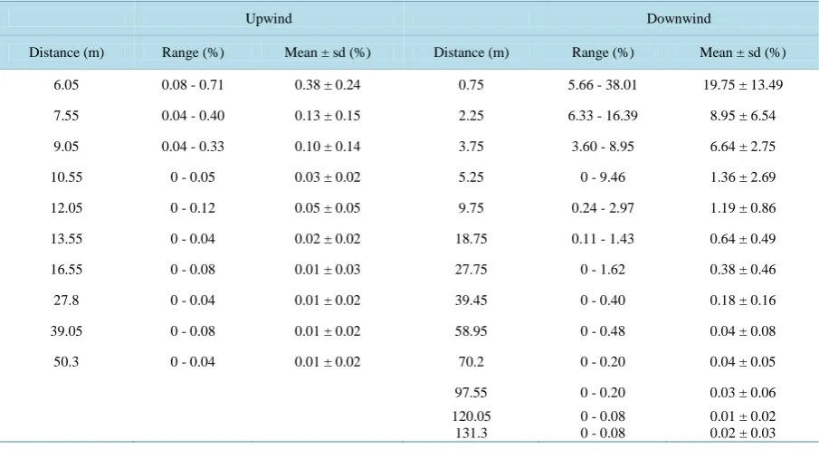
Table 2 shows the ranges and average CP rates in various directions and distances for the first crop season. As expected, the CP rate was highest in the first row of the recipient field adjacent to the source plot. Although the average CP rate 0.75 m from the source plot was only 6.07% downwind compared to 6.33% in the upwind di-rection, the majority of the higher average CP rates were observed downwind rather than upwind. The extent of the CP rate in the subsequent rows declined rapidly farther from the source plot. In the upwind direction, low levels (0% - 0.24%) of CP rates were recorded at 15 m, and decreased to 0% thereafter. However, in the down-wind direction, a 0% to 0.24% CP rate was recorded at 28.5 m. The average CP rate reached 0% at 29.25 m, but the average was 0.08% (0% - 0.49%) at 30 m. The average CP rate in the downwind direction was higher in the second crop season (19.75%) than in the first crop season (6.07%), and the CP rate declined when distances in-creased from the source plot (Table 2, Table 3). In the upwind direction, the average CP rate at 6.05 m from the source plot was 0.38% and decreased in the subsequent rows. The average CP rate was never 0% within 50.3 m and 131.3 m where samples were collected in upwind and downwind directions, respectively (Table 3).

In the first crop season, the average CP rates were approximately 5.32% - 6.40% from 0 to 3 m (Table 4). The average CP rates were greater in the east and south than in the west and north. Similarly, a greater distance from the source plot indicated a lower CP rate. At a distance of 10 - 20 m, the average CP rates were higher in the south (0.34%) than in the north (0.06%) and were higher in the east (0.07%) than in the west (0.02%). The re-sults are consistent with the wind direction of NW. In the second crop season, the average CP rates were 11.69% in the east and 15.70% in the south compared to 0.34% in the north and 3.19% in the west at 0 - 3 m (Table 5). Similar patterns were observed at distances of 20 - 25 m. The average CP rate was 0% beyond 50 m in the first crop season but was never 0% within 131.3 m in the second crop season (Table 4, Table 5).

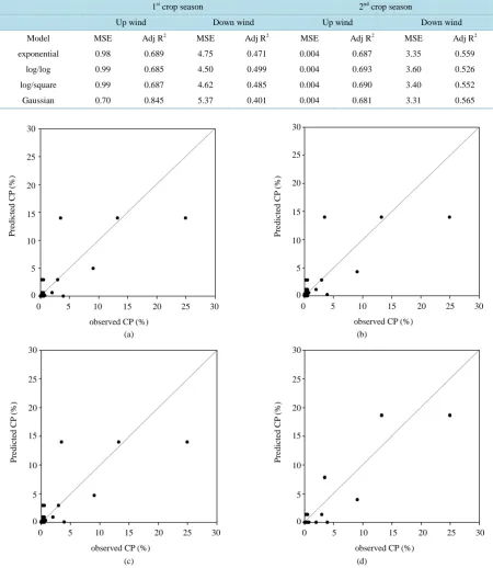
3.4. Performance of the Gene Flow Models

Three empirical models and one semi-empirical model were used to predict the CP rates at various distances,

Table 2.Mean and range of cross-pollination rate (%) in the first crop season.

Upwind Downwind

Distance (m) Range (%) Mean ± sd (%) Distance (m) Range (%) Mean ± sd (%)

0.75 0 - 24.94 6.33 ± 9.02 0.75 0 - 25.92 6.07 ± 8.25

1.5 0 - 2.93 0.73 ± 1.25 1.5 0 - 4.16 1.52 ± 2.00

2.25 0 - 1.96 0.54 ± 0.82 2.25 0 - 0.98 0.31 ± 0.46

3 0 - 0.73 0.29 ± 0.32 3 0 - 2.44 0.67 ± 1.19

3.75 0 - 0.24 0.05 ± 0.11 3.75 0 - 8.07 3.33 ± 4.33

4.5 0 - 3.91 0.17 ± 0.70 4.5 0 - 5.87 2.10 ± 2.57

7.5 0 0.00 10.5 0 - 1.96 0.18 ± 0.39

15 0 - 0.24 0.05 ± 0.11 20.25 0 - 1.96 0.10 ± 0.33

24 0 0.00 28.5 0 - 0.24 0.05 ± 0.11

68 0 0.00 29.25 0 0.00

98 0 0.00 30 0 - 0.49 0.08 ± 0.20

Table 3. Mean and range of cross-pollination rate (%) in the second crop season.

Upwind Downwind

Distance (m) Range (%) Mean ± sd (%) Distance (m) Range (%) Mean ± sd (%)

6.05 0.08 - 0.71 0.38 ± 0.24 0.75 5.66 - 38.01 19.75 ± 13.49

7.55 0.04 - 0.40 0.13 ± 0.15 2.25 6.33 - 16.39 8.95 ± 6.54

9.05 0.04 - 0.33 0.10 ± 0.14 3.75 3.60 - 8.95 6.64 ± 2.75

10.55 0 - 0.05 0.03 ± 0.02 5.25 0 - 9.46 1.36 ± 2.69

12.05 0 - 0.12 0.05 ± 0.05 9.75 0.24 - 2.97 1.19 ± 0.86

13.55 0 - 0.04 0.02 ± 0.02 18.75 0.11 - 1.43 0.64 ± 0.49

16.55 0 - 0.08 0.01 ± 0.03 27.75 0 - 1.62 0.38 ± 0.46

27.8 0 - 0.04 0.01 ± 0.02 39.45 0 - 0.40 0.18 ± 0.16

39.05 0 - 0.08 0.01 ± 0.02 58.95 0 - 0.48 0.04 ± 0.08

50.3 0 - 0.04 0.01 ± 0.02 70.2 0 - 0.20 0.04 ± 0.05

97.55 0 - 0.20 0.03 ± 0.06

120.05 131.3

0 - 0.08 0 - 0.08

0.01 ± 0.02 0.02 ± 0.03

Table 4. Rate of cross-fertilization (%) at each direction (N, S, W, E) in the first crop season.

Distance (m) 1st crop season Avg

N S W E

0 - 3 5.32 ± 8.41 6.40 ± 8.00 5.40 ± 8.91 5.55 ± 7.19 5.64

3 - 6 0.15 ± 0.22 2.61 ± 3.34 0.09 ± 0.14 0.82 ± 1.07 0.61

10 - 20 0.06 ± 0.15 0.34 ± 0.54 0.02 ± 0.17 0.07 ± 0.34 0.06

20 - 30 0.00 0.03 ± 0.08 n.d. n.d. 0.04

50 - 60 0.00 n.d.a _{n.d. n.d. 0.00}

90 - 100 0.00 n.d. n.d. n.d. 0.00

a_{no data collected.}

Table 5. Rate of cross-fertilization (%) at each direction (N, S, W, E) in the second crop season.

Distance (m) 2nd _{crop season Avg}

N S W E

0 - 3 0.34 ± 0.24 15.70 ± 12.14 3.19 ± 4.65 11.69 ± 8.95 8.00

3 - 6 0.06 ± 0.11 7.00 ± 4.25 0.15 ± 0.22 1.63 ± 0.86 2.42

6 - 9 0.03 ± 0.04 2.80 ± 0.74 0.13 ± 0.13 0.52 ± 0.39 0.89

20 - 25 0.01 ± 0.02 0.66 ± 0.40 0 0.13 ± 0.12 0.24

35 - 40 0.01 ± 0.02 0.57 ± 0.46 n.d. n.d. 0.06

70 - 80 n.d.a _{0.04 ± 0.05 n.d. n.d. 0.03}

120 - 131.3 n.d. 0.01 ± 0.02 n.d. n.d. 0.01

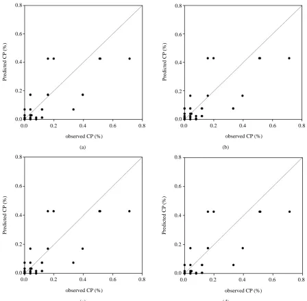
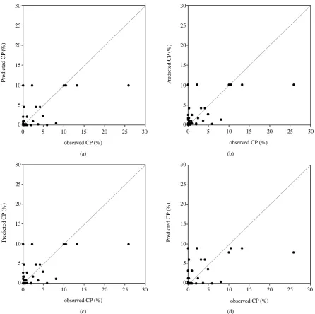
and the suitability of these models were compared (Table 6). Considering the upwind direction, data for the first crop season fitted by the Gaussian Plume model performed best with the largest R2 value and the smallest MSE (adj. R2 = 0.845, MSE = 0.7). However, the log/log model had the best fitting ability in the second crop season (adj. R2 = 0.693, MSE = 0.004). The relationship among the predicted verse measured CP rates showed the same tendency (Figure 4, Figure 5). The Gaussian Plume model had the largest r value of 0.92 in the first crop

Table 6. Mean squared error (MSE), adjusted coefficient of determination (adj R2) of the four models in both crop seasons.

1st _{crop season 2}nd _{crop season}

Up wind Down wind Up wind Down wind

Model MSE Adj R2 MSE Adj R2 MSE Adj R2 MSE Adj R2

exponential 0.98 0.689 4.75 0.471 0.004 0.687 3.35 0.559

log/log 0.99 0.685 4.50 0.499 0.004 0.693 3.60 0.526

log/square 0.99 0.687 4.62 0.485 0.004 0.690 3.40 0.552

Gaussian 0.70 0.845 5.37 0.401 0.004 0.681 3.31 0.565

observed CP (%)

P

red

ict

ed

C

P

(

%

)

0 0 10 20 30

10 15 20 25 30 5

25

15

5

observed CP (%)

P

red

ict

ed

C

P

(

%

)

0 0 10 20 30

10 15 20 25 30 5

25

15

5

(a) (b)

observed CP (%)

P

red

ict

ed

C

P

(

%

)

0 0 10 20 30

10 15 20 25 30 5

25

15

5

observed CP (%)

P

red

ict

ed

C

P

(

%

)

0 0 10 20 30

10 15 20 25 30 5

25

15

5

(c) (d)

observed CP (%)

P

red

ict

ed

C

P

(

%

)

0.0 0.0

0.2 0.4 0.6 0.8

0.2 0.4 0.6 0.8

observed CP (%)

P

red

ict

ed

C

P

(

%

)

0.0 0.0

0.2 0.4 0.6 0.8

0.2 0.4 0.6 0.8

(a) (b)

observed CP (%)

P

red

ict

ed

C

P

(

%

)

0.0 0.0

0.2 0.4 0.6 0.8

0.2 0.4 0.6 0.8

observed CP (%)

P

red

ict

ed

C

P

(

%

)

0.0 0.0

0.2 0.4 0.6 0.8

0.2 0.4 0.6 0.8

(c) (d)

Figure 5. Scatter plots of observed and model-estimated cross-pollination rate in upwind direction in the second crop season (n = 115). (a) Exponential (r = 0.83); (b) Log/log (r = 0.84); (c) Log/square (r = 0.84); (d) Gaussian plume model (r = 0.83).

observed CP (%)

P

red

ict

ed

C

P

(

%

)

0 0 10 20 30

10 15 20 25 30 5

25

15

5

observed CP (%)

P

red

ict

ed

C

P

(

%

)

0 0 10 20 30

10 15 20 25 30 5

25

15

5

(a) (b)

observed CP (%)

P

red

ict

ed

C

P

(

%

)

0 0 10 20 30

10 15 20 25 30 5

25

15

5

observed CP (%)

P

red

ict

ed

C

P

(

%

)

0 0 10 20 30

10 15 20 25 30 5

25

15

5

(c) (d)

Figure 6. Scatter plots of observed and model-estimated cross-pollination rate in downwind direction in the first crop season (n = 136). (a) Exponential (r = 0.69); (b) Log/log (r = 0.71); (c) Log/square (r = 0.70); (d) Gaussian plume model (r = 0.64).

observed CP (%)

P

red

ict

ed

C

P

(

%

)

0 10 20 30 40

0 10 20 30 40

observed CP (%)

P

red

ict

ed

C

P

(

%

)

0 10 20 30 40

0 10 20 30 40

(a) (b)

observed CP (%)

P

red

ict

ed

C

P

(

%

)

0 10 20 30 40

0 10 20 30 40

observed CP (%)

P

red

ict

ed

C

P

(

%

)

0 10 20 30 40

0 10 20 30 40

(c) (d)

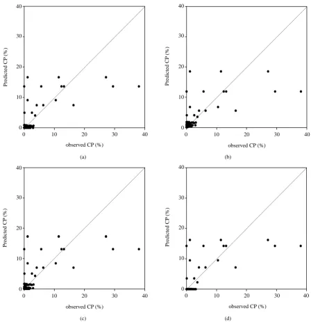
Figure 7. Scatter plots of observed and model-estimated cross-pollination rate in downwind direction in the second crop season (n = 522). (a) Exponential (r = 0.75); (b) Log/log (r = 0.73); (c) Log/square (r = 0.74); (d) Gaussian plume model (r = 0.75).

4. Discussion

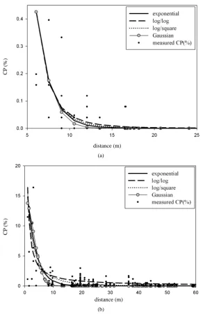
In the first report of this study, it was observed that the CP rate declined rapidly with increasing distance from the source field. The CP rates at short distances were more variable. These results are in agreement with those from other studies [2] [6]-[11]. The CP rates of the recipients were well fitted by the four models in this study. However, the samples with higher CP rates adjacent to the pollen source were underestimated when using these models. In contrast, Loos et al. [7] observed tendencies in overestimation using the Gaussian Plume model and LNF theory on their data in farther distances from the source field.

distance (m)

C

P (

%

)

(a)

distance (m)

C

P (

%

)

(b)

Figure 8. Scatter plots of observed (dot) and model-estimated (line) cross-pol- lination (%) in the first crop season. (a) Upwind direction; (b) Downwind di-rection.

natural barrier and competitor for the source pollen. Apart from the relative sizes of the source and recipient fields, the wind direction and average wind speed in the second crop season provided favorable conditions for achieving higher CP rates. These results are consistent with the work of Ma et al. [2] who reported that the CP rates were <1% at a distance of 28 m downwind, but at a distance of 10 m upwind in all sites and years tested.

distance (m)

C

P (

%

)

(a)

distance (m)

C

P (

%

)

(b)

Figure 9. Scatter plots of observed (dot) and model-estimated (line) cross-pol- lination (%) in the second crop season. (a) Upwind direction; (b) Downwind direction.

None of the models used in this study were excellent in simulating the field data because the R2 values were not large, which indicated that biological (e.g., the height of male and female flowers) and aerodynamic factors (e.g., wind speed, wind direction, pollen settling velocity, and air turbulence) must be considered when model-ing gene flow. The CP rates of the recipient at various distances from the source are well fitted by the Gaussian Plume model compared with other empirical models. Therefore, future works should introduce important bio-logical, agricultural, and climatic parameters into proposed models to test the influence of these parameters on maize gene flow, and to create a more useful maize gene flow model.

5. Conclusion

This study was the first to construct the field experiment in Taiwan to measure the CP rate for simulating the GM maize. By using phenotypic marker and determining the isolation distance between the 2 maize varieties, this study detected the effects on the CP rate of maize at a field-scale level. Accordingly, the results showed that the CP rate was affected by distance, area ratio of source and recipient, wind direction, and synchrony of flo-wering time. It is effective to maintain a CP rate below 0.9% without any additional temporal isolation by sur-rounding pollen sources with ranges of isolation distances between 10 and 50 m. Moreover, the Gaussian Plume model fitted better than the other empirical models. However, the small scale of agricultural landscapes is one common situation in Taiwan which has a subtropical insular climate. Therefore, meteorological elements and biotic factors must be considered for investigating the gene flow in Taiwan to further improve the performance of model fitting and prediction.

References

[1] James, C. (2013) Global Status of Commercialized Biotech/GM Crops: 2012. ISAAA Brief, ISAAA, Ithaca.

[2] Ma, B.L., Subedi, K.D. and Reid, L.M. (2004) Extent of Cross-Fertilization in Maize by Pollen from Neighboring Transgenic Hybrids. Crop Science, 44, 1273-1282. http://dx.doi.org/10.2135/cropsci2004.1273

[3] Palaudelmás, M., Melé, E., Peñas, G., Pla, M., Nadal, A., Serra, J., Salvia, J. and Messeguer, J. (2008) Sowing and Flowering Delays Can Be an Efficient Strategy to Improve Coexistence of Genetically Modified and Conventional Maize. Crop Science, 48, 2404-2413.

[4] Marceau, A., Loubet, B., Andrieu, B., Dur, B., Foueillassar, X. and Huber, L. (2011) Modeling Diurnal and Seasonal Patterns of Maize Pollen Emission in Relation to Meteorological Factors. Agricultural and Forest Meteorology, 151, 11-21. http://dx.doi.org/10.1016/j.agrformet.2010.08.012

[5] Devos, Y., Demont, M., Dillen, K., Reheul, D., Kaiser, M. and Sanvido, O. (2009) Coexistence of Genetically Mod-ified (GM) and Non-GM Crops in the European Union. A Review. Agronomy for Sustainable Development, 29, 11-30.

http://dx.doi.org/10.1051/agro:2008051

[6] Luna, S.V., Figueroa, J.M., Baltazar, B.M., Gomez, R.L., Townsend, R. and Schoper, J.B. (2001) Maize Pollen Lon-gevity and Distance Isolation Requirements for Effective Pollen Control. Crop Science, 41, 1551-1557.

http://dx.doi.org/10.2135/cropsci2001.4151551x

[7] Loos, C., Seppelt, R., Meier-Bethke, S., Schiemann, J. and Richter, O. (2003) Spatially Explicit Modeling of Trans- genic Maize Pollen Dispersal and Cross-Pollination. Journal of Theoretical Biology, 225, 241-255.

http://dx.doi.org/10.1016/S0022-5193(03)00243-1

[8] Gustafson, D.I., Horak, M.J., Rempel, C.B., Metz, S.G., Gigax, D.R. and Hucl, P. (2005) An Empirical Model for Pol- len-Mediated Gene Flow in Wheat. Crop Science, 45, 1286-1294. http://dx.doi.org/10.2135/cropsci2004.0137

[9] Halsey, M.E., Remund, K.M., Davis, C.A., Qualls, M., Eppard, P.J. and Berberich, S.A. (2005) Isolation of Maize from Pollen-Mediated Gene Flow by Time and Distance. Crop Science, 45, 2172-2185.

http://dx.doi.org/10.2135/cropsci2003.0664

[10] Messeguer, J., Penas, G., Ballester, J., Bas, M., Serra, J., Salvia, J., Palaudelmas, M. and Mele, E. (2006) Pollen-Me- diated Gene Flow in Maize in Real Situations of Coexistence. Plant Biotechnology Journal, 4, 633-645.

http://dx.doi.org/10.1111/j.1467-7652.2006.00207.x

[11] Della Porta, G., Ederle, D., Bucchini, L., Prandi, M., Verderio, A. and Pozzi, C. (2008) Maize Pollen Mediated Gene Flow in the Po Valley (Italy): Source-Recipient Distance and Effect of Flowering Time. European Journal of Agrono- my, 28, 255-265. http://dx.doi.org/10.1016/j.eja.2007.07.009

[12] Frederick, C. (2011) Taiwan Biotechnology Annual Report. USDA Foreign Agricultural Service.

[13] Pasquill, F. (1974) Atmospheric Diffusion, 2nd Edition, Wiley, New York.

[14] Yao, K., Hu, N., Cheng, W., Li, R., Yuan, Q., Wang, F., Qian, Q. and Jia, S. (2008) Establishment of a Rice Transgene Flow Model for Predicting Maximum Distances of Gene Flow in Southern China. New Phytologist, 180, 217-228.

http://dx.doi.org/10.1111/j.1469-8137.2008.02555.x

[15] Neter, J., Kutner, M.H., Nachtsheim, C.J. and Wasserman, W. (1996) Applied Linear Statistical Models. 4th Edition, McGraw-Hill Professional Publishing, New York.

[16] Aylor, D.E., Schultes, N.P. and Schields, E.J. (2003) An Aerobiological Framework for Assessing Cross-Pollination in Maize. Agricultural and Forest Meteorology, 119, 111-129. http://dx.doi.org/10.1016/S0168-1923(03)00159-X

[17] Jarosz, N., Loubet, B., Durand, B., Foueillassar, X. and Huber, L. (2005) Variations in Maize Pollen Emission and Deposition in Relation to Microclimate. Environmental Science & Technology, 39, 4377-4384.