A Fractal Space Time Structure of Nonequilibrium Living Systems Is Essential Property and Fractal Property of Dynamics Systems on Cosmic Scales Is Foundation for the Origin of the Living Systems

http://dx.doi.org/10.4236/ojbiphy.2014.42007

A Fractal Space-Time Structure of

Nonequilibrium Living Systems Is Essential

Property and Fractal Property of Dynamics

Systems on Cosmic Scales Is Foundation for

the Origin of the Living Systems

Victor Gusev1,2,3,4

1_{Sobolev Institute of Mathematics, Siberian Branch, Russian Academy of Sciences, Novosibirsk, Russia} 2_{Institute Cytology and Genetics Siberian Branch, Russian Academy of Sciences, Novosibirsk, Russia} 3_{Novosibirsk State University, Novosibirsk, Russia}

4_{Institute Laser Physics Siberian Branch, Russian Academy of Sciences, Novosibirsk, Russia}

Email: [email protected]

Received 11 December 2013; revised 13 January 2014; accepted 20 January 2014

Copyright © 2014 by author and Scientific Research Publishing Inc.

This work is licensed under the Creative Commons Attribution International License (CC BY).

http://creativecommons.org/licenses/by/4.0/

Abstract

The experimental data represented in the bibliography are theoretically analyzed to construct an adequate model for dynamics of an open nonequilibrium living system. It is shown that the viable microorganisms are capable of forming the fractal structure, whose dimensionality is certainly non-integral. In addition, we have attempted to provide a generalized description of the proper-ties of living and nonliving matter (in the addition to that described in work [1]). Relevant pub-lished data were used to demonstrate a fractal structure of the space in the vicinity of centrally gravitating bodies with satellites revolving around them along closed trajectories and serving as a kind of testers of the neighboring space. A local violation of its discontinuity is likely to be a ne-cessary (yet not sufficient!) dynamic characteristic of the spatiotemporal continuum for self-or- ganization of molecules into a living, i.e., self-replicating, system.

Keywords

1. Introduction

Over 50 years ago, two Moscow microbiologists, V.A. Elin and V.O. Kalinenko, independently from one another discovered a paradoxical phenomenon, namely, the ability of organotrophic microbial E. coli cells after a certain pretreatment to reproduce in the saline solutions completely deprived of any organic substances. Inde-pendently of the composition of this saline solution (be it physiological solution or phosphate buffer) and the in-itial concentration of viable cells (103 - 105 cm–3), all populations over 1 - 2 days of incubation at 37˚C reached the same limit concentration of about 106 cm–3 and retained a long-term viability in this state without any access to organics. Results of these experiments were published in the journal Mikrobiologiya (Microbiology) [2] [3]. This phenomenon has not been explained in any manner acceptable for microbiologists, being regarded as an ar-tifact, and was forgotten for years.

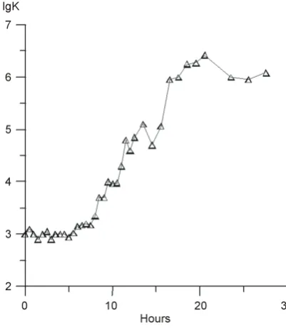
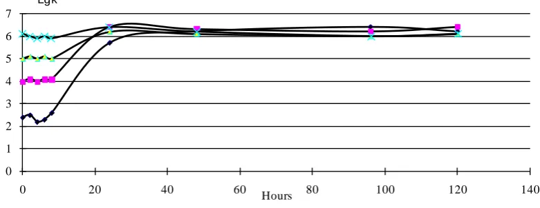
Thirty years ago, our research team by a lucky confluence of circumstances discovered an analogous pheno-menon of reproduction of an organotrophic microorganism, E. coli, under even more stringent conditions, in te-tradistilled water. These experiments are described in [4]-[10] and also in monograph [11]. There we also for-mulated a biophysical model for this phenomenon. Additional experimental data on the evolutionary drift of the number of viable cells (hereinafter, NVC), cooperative effects, quasiperiodic variations of the mean NVC value in a sample, as well as relative variance and biorhythms in the microbial communities under extreme conditions of absolute substrate starvation, i.e., in a superpure distilled water, are briefed in [7] [9]. Below, we describe the results of further studies into the properties of microbial populations in a substrate-free medium. Here we will present only some experimental data. Figure 1 and Figure 2 represent the dynamics of the multiplication of mi-croorganisms of E. coli in the distilled water.

2. Nonlinear Phenomena in Microbial Population Dynamics

It is easy to calculate, that the quantity of organic substratum, necessary for the amplification of cells 103 - 104 times cannot be contained as the spare substances in the polysaccharide capsule or the walls of initial cells. Fur-thermore, as showed authors [12] (these given they were confirmed in our studies), the cell of microorganisms under these conditions they do not lose the ability to be multiplied during repeated multiplication in the distilled water—which completely excludes the possibility of use by microorganisms the residual spare substances of

Figure 1. Amplification of the cells of E. coli in the dis-tilled water. Along the Y-axis the common logarithm of cell concentration in ml, the temperature of the incubation of 37˚C, the time of the doubling of cells, averaged in the

Figure 2.Independence of the final steady state of population from the initial concentration of cells. Along

the Y-axis the common logarithm of concentration of cells in ml, the temperature of the incubation of 22˚C.

cellular components for the reproduction of daughterly cells. Here one should again note that independent of the degree of the isolation of cells from the possible sources of organic substrata, in all works indicated the authors observed one general regularity. With the arbitrary initial concentration of cells from 102 to 106 cm−3 final con-centration in 1 - 2 days of incubation at a temperature of 22˚C - 37˚C composed (2 - 5) × 106

cm−3 (Figure 1, Figure 2).

In our works [4]-[11] is for the first time formulated the biophysical model of this phenomenon of the ampli-fication of microorganisms in “absolute clear water”. Work [9] additionally presents the experimental data about the evolutionary drift of the number of viable cells (further NVC), the cooperative effects, quasi-periodic varia-tions in the average value NVC in the model, and so to relative dispersion and biorhythms in the microbial asso-ciations, which are located in the extreme conditions of absolute substrate hunger, i.e., in the super-clean distill-ed water. Are representdistill-ed below the results of further of the examination of the properties of the populations of microorganisms in the clear water.

Let us begin the analysis of nonlinear effects in the population of the living systems of microorganisms from the completely nontrivial phenomenon—the disturbance “elementary statistical regularities”. In Figure 3 is represented the dependence of the relative dispersion of 2

k

σ from the time.

The first, what does cause surprise and does raise the question—why relative dispersion does vary, at that time when on the conditions for experiment it must be constant? Moreover, according to laws the statisticians Poisson (namely to this statistics must be subordinated the distribution of microorganisms on the separate tests in accordance with the procedure of setting experiment!) 2

1 k

σ ≡ .

Hence follows the obvious conclusion: the population of living i.e., nonequilibrium systems is permanently reconstructed in the space in such a way that tendency toward the regular order, when 2

1 k

σ < it is changed to “super-chaos” with 2

1 k

σ > . This state of the set of discrete nonequilibrium systems or cells of microorgan-isms can be represented as the hierarchy of clusters “by living at the given instant” molecular structure with in-active for some time, but integral and potentially in-active molecular structure.

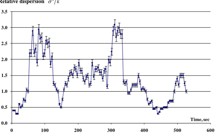
It is extremely important to note that this phenomenon is not connected directly with the displacement in the space of molecular structures, i.e., the cells of microorganisms. We specially conducted the examination of our own mobility of microorganisms in the given specific conditions and showed that the speed of their three-di- mensional displacement does not exceed 50 mkm/sec [13], i.e., moving with such speeds in the volume of liquid, the cells of microorganisms will not have time for 100 - 200 sec it flogged to create in the space the regulated or “super-chaotic” clusters of discrete molecular structures. It is lower in Figure 4 are represented the experimental data about a variation in the relative dispersion in the interval of measurement per second.

Comparing these data and maximum mobility of the cells of microorganisms, it is possible to draw the sin-gle-valued conclusion that variations in the relative dispersion on such temporary scales cannot be provide ford only due to the three-dimensional displacement of the molecular structures of cells as whole.

To explain such sufficiently regular variations in the relative dispersion on the different temporary scales possible, if one assumes that on molecular many potentially “viable” objects is formed the self-similar fractal structure, whose nature, apparently, is not molecular, but is sooner anything field-electromagnetic or gravita-

0 1 2 3 4 5 6 7

0 20 40 60 80 100 120 140

Lgk

Relative dispersion 2

k σ

Figure 3.Temporary evolution of relative dispersion. Concentration of the viable cells of K =

940 ± 30 cm−3.

Relative dispersion σ2 _k

Figure 4.Variations in the relative dispersion on short times’ intervals. Tests from the initial

volume of population with the concentration of ≈4 × 103 cm−3 were selected with the interval of

0.5 sec.

tional there is no as yet single-valued answer. One is clear—these structures cannot be stationary and equili-brium. This is the first difficultly refutable conclusion, which follows from represented experimental data.

Let us be distracted for some time from variations in the relative dispersion, and let us examine nonlinear ef-fects in the population of the microorganisms.Figure 5 shows the dependences of NVC on the sampling volume taken from the initial population.

The initially linear dependence for small sampled volumes deviates from a linear pattern in a statistically sig-nificant manner with increase in this volume. The value and pattern of such deviations are not strictly fixed for an individual sample in population yet change with time (see Figure 11).

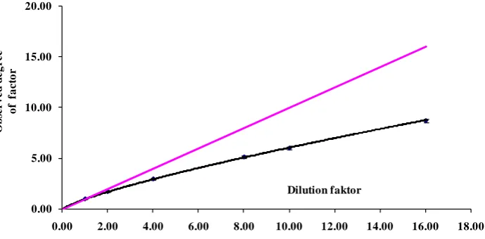
Consider one more nonlinear effect associated with a change in concentration of microbial suspension with its dilution with water (Figure 6). It could be a priori expected that an m-fold dilution of the suspension containing K0 cells per unit volume will change the cell as:

0.00 0.20 0.40 0.60 0.80 1.00 1.20 1.40 1.60

0.00 20.00 40.00 60.00 80.00 100.00 120.00 140.00 160.00 180.00 200.00 Time, min

0.0 0.5 1.0 1.5 2.0 2.5 3.0 3.5

0 100 200 300 400 500 600

Figure 5.Nonlinear dependence of the number of viable cells in sampled volume. The or-dinate shows the NVC in sample.

Figure 6. Nonlinear dependence of concentration on dilution factor. Nonlinearity coefficientα =

0.783 ± 0.023; correlation coefficient of nonlinear approximation r = 0.999; and solid line, linear

approximation according to initial data.

o th m

K m

K = , (1)

where denominator is the theoretically expected value of microbial concentration. However, the experimental data transform this dependence to:

exp

o

m

K m K

α

= (2)

where denominator is the experimentally observed microbial concentration.

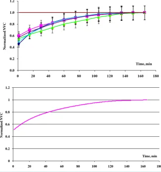
The nonlinearity coefficient α is not a strictly fixed constant. Its value is mainly determined by the time of re-laxation to stationary state after mechanical disturbance of population (see Figure 7).

Figure 7 shows the experimental dependence of a change in NVC after dilution of the initial concentrated suspension (K ≈ 108

cm–3) to the concentration K ≈ 103 cm–3. Within the error, the parameters of relaxation curve are independent of the degree of population dilution.

Note that immediately after dilution of cell suspension, NVC drops strictly twofold independently of the dilu-tion factor and then again relaxes to the initial concentradilu-tion. Evidently, there is no quesdilu-tion of any irreversible mechanical destruction of half cell population. Presumably, after a mechanical disturbance of population, a rapid destruction of autonomously stable spatial population structure takes place with its subsequent slow relaxation to

0 20 40 60 80 100 120 140

0 20 40 60 80 100 120

K

Volume, mkl

0.00 5.00 10.00 15.00 20.00

0.00 2.00 4.00 6.00 8.00 10.00 12.00 14.00 16.00 18.00

Dilution faktor

O

b

se

rv

e

d

d

eg

r

ee

o

f

fa

c

to

Figure 7. Relaxation of the number of viable cells (NVC) in water at a room temperature after dilution of the initial suspension. The initial population with a concentration of viable

cells of ~108 cm–3was kept at +4˚C for 2 days to immediately (for 5 - 7 min) prepare five

tenfold dilutions (initial suspension with 108 cm–3; next series 107 cm–3, 106 cm–3, 105 cm–3,

104 _cm–3 _and103 _cm–3_{) with distilled water at a room temperature and sample them}

periodi-cally for determining NVC. The NVC value (the ordinate) was normalized by dividing the

NVC at a given moment by stationary NVC value (upper curves). Averaging was

per-formed over all dilutions (see upper curves). The approximation curve K/K0 = 1 –

0.5exp(–t/42.7) with the correlation coefficient r _{= 0.8; relaxation time} τ = 42.7 min.

the state that provides all cells with the amount of free environmental energy sufficient for maintaining the via-bility of the entire population.

The experimental data suggest that:

• Nonlinear phenomena are observed when sampling the population with a constant cell concentration, name-ly, the NVC in samples increases not directly proportionally to their volume;

• The change in NVC is also not directly proportional to the dilution factor after changing cell concentration (diluting cell suspension via addition of water);

• The spatial structure of population is rather sensitive to external mechanical disturbance but is able to relax to the initial state.

To determine the physical meaning of nonlinearity coefficients, we use fractal geometry methods. As is known, the objects of fractal geometry are the structures with a characteristic hierarchy and a scale invariance.

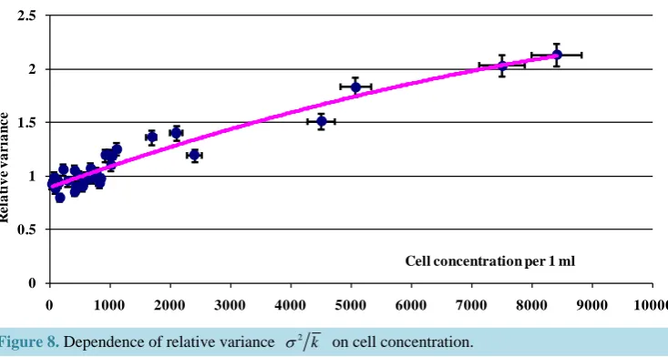
See Figure 8, which shows the dependence of the relative variance 2

T

k

σ averaged over time at various cell concentrations (the mean NVC value in sample k is proportional to the mean cell concentration K, be-cause the samples of strictly fixed volume were taken; σ , the variance in series of samples). The time intervals of averaging were changed in a random manner from point to point in the range of (1 - 4) h. This processing

0.0 0.2 0.4 0.6 0.8 1.0 1.2

0 20 40 60 80 100 120 140 160 180

No

r

m

a

li

z

e

d

NVC

Time, min

0 0.2 0.4 0.6 0.8 1 1.2

0 20 40 60 80 100 120 140 160 180

N

o

rm

a

li

zed

N

V

C

Relative variance 2

k σ

Figure 8.Dependence of relative variance σ2 _{k on cell concentration.}

method was selected to level the accuracy error inevitably introduced when counting NVC.

These data suggest that a cell concentration of 8 × 102 cm–3 is the critical point below which the variance 2 _{k 1}

σ < ; with increase in cell concentration, the relative variance exceeds unity and even permanently grows. This effect can be interpreted as a transition from quasi-regulated distribution of viable cells at concentrations below 8 × 102 cm–3 in the volume to heterogeneous distribution, when a hierarchy of clusters with different concentrations of viable cells is formed. In addition, a complex evolution of these clusters is observed. This conclusion was made based on the variations of relative variance around the mean value with time; this mean value is determined by the concentration of viable cells (see Figure 3 and Figure 4).

Without getting into the physical mechanism of this phenomenon, consider its formal aspect. In the case of a hierarchical self-similar distribution of elementary units forming a fractal object in three-dimensional Euclidean space, their density in a volume is not a constant but rather depends on the sample volume as follows:

( )

D

o o

V V

V

ρ ρ

−

 

= _{ }

  (4)

where ρ

( )

den-sity over the entire volume occupied by fractal object; Vo, the volume of one elementary unit (in this case, the

volume per one cell, a uniform distribution of the overall population provided); and DR, fractal dimensionality of

the object. It follows from Equation (4) that at m-fold dilution of the population displaying fractal properties, the corresponding densities ρ

( )

( )

( )

( )

D

m V

m V

ρ

ρ = (5).

As it follows from Equations (2) and (5), the fractal dimensionality and nonlinearity coefficient are related as: 3

D= α. (6) Figure 9 shows the dependence of fractal dimensionality on the concentration of microorganisms calculated using this equation.

At a cell concentration exceeding 3 × 103 cm–3, the curve in figure commences significantly deviating from asymptotic value of 3, characteristic of small concentrations.

3. Relaxation Dynamics of Fractal Dimensionality

Figure 10 shows the relaxation curve for fractal dimensionality of microbial population after mechanical dis-turbance.

0 0.5 1 1.5 2 2.5

0 1000 2000 3000 4000 5000 6000 7000 8000 9000 10000

R

e

la

ti

v

e

v

a

r

ia

n

c

e

Figure 9.Dependence of fractal dimensionality on the concentration of viable cells. The abscissa shows the

decimal logarithm of cell concentration per 1 cm3.

Figure 10.Dependence of the fractal dimension of population on the relaxation time after mechanical

distur-bance. Concentration of suspension is (3.5 ± 0.07) × 103 cm–3.

The essence of experiment was as follows: suspension of microbial cells was intensively stirred and then, as soon as possible (as a rule, over 15 - 20 s), 5 ml of this mechanically disturbed suspension was pumped using a peristaltic pump into a separate glass container (tube). Then samples were taken from this tube and multiply di-luted with water (as a rule with a step of two). The didi-luted samples were plated onto Petri dishes containing agar nutrient medium to determine the concentration of viable cells. The dishes were incubated overnight at 37˚C to count the colonies on the next day and determine the fractal dimensionality using Equation (6).

As is evident from Figure 10, the mechanically disturbed population completely relaxed to the stationary value of fractal structure over more than 15 min. It was necessary to take this fact into account when determin-ing the dimensionality D for the population exposed to mechanical disturbance, for example, after dilution.

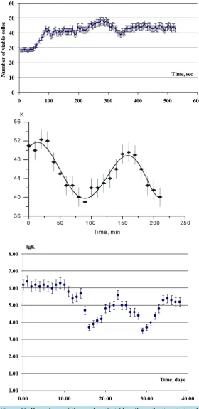
To construct a self-consistent spatiotemporal model for living systems, we then need the experimental data on the time drift and dynamics of microbial populations. As has been demonstrated [4]-[11], it is almost impossible to observe a living system in a stationary state. For the observation times from seconds to several days when the

2.0 2.2 2.4 2.6 2.8 3.0 3.2 3.4

0.0 0.5 1.0 1.5 2.0 2.5 3.0 3.5 4.0

F

rac

tal

d

ime

n

si

on

al

ity D

log K

2.74 2.76 2.78 2.8 2.82 2.84 2.86 2.88 2.9 2.92

0.00 2.00 4.00 6.00 8.00 10.00 12.00 14.00 16.00

F

r

a

c

ta

l d

im

e

n

ti

o

n

population of organotrophic microorganisms in a substrate-free medium was monitored, the NVC permanently varied by tens of percent from the mean value (for small times) to several orders of magnitude and back to the mean value at long times (see Figure 11). In other words, it is also possible to introduce the concept of a time fractal for populations of the living systems that form a spatial fractal structure [14] [15].

4. A Fractal Structure of Space and Time in Living Systems

In both the everyday live and scientific research, it is a priori considered that the space where we live has integ-er dimensionalities: line is one-dimensional, plane is two-dimensional, and space has only three dimensions. It seems that it is impossible to imagine the world and the objects in it with fractional dimensionalities. However, this is a mere consequence of our conservatism and habits. A coastline, clouds, porous structures, electrical dis-charges in atmosphere, and many other natural phenomena are much easier describable with the help of the lan-guage of mathematical equations by introducing the concept of fractality, i.e., a fractional dimensionality. The branched network of blood vessels of warm-blooded animals as well as their neuronal network, branching structures of trees, and so on can be described in an analogous manner. It appeared a surprising fact for us that the distribution of viable aquatic microbial cells in a volume can also be described using the language of fractals. Figure 6 shows the approximation of experimental data with the nonlinearity coefficient α = 0.78 ± 0.02. These data make it possible to determine the fractal dimensionality of theset of viable cells distributed in popu-lation volume as D = 2.35 ± 0.07.

The fractal dimensionality of time is determined when analyzing long-term time variations in NVC in micro-bial population via the Hurst constant [15]. This constant is determined as:

(

)

max min ln

ln 2

K K

H

T t

σ

−

= (7)

where Kmax and Kmin are the maximal and minimal NVC in the array of samples taken during the time T with an interval t and σ, the variance for this array. The number of samples in the array, N=T t, in our experiments was no less than 600, because it was demonstrated beforehand that the Hurst constant in such array reached a stationary value, which could be later used for calculating the fractal dimensionality of time using the equation from [15]:

2

T

D = −H, (8)

where DT is the fractal dimensionality of time for the data array.

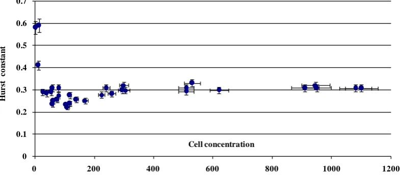
Figure 12 demonstrates the dependence of the Hurst constant on concentration of viable cells. Here each point was obtained based on 600 - 800 samples taken from population with a fixed cell concentration.

It is easy to calculate the fractal dimensionality of population, DT = 2 – Hst(K) = 2 – 0.309 = 1.691 ± 0.004.

A formal description of objects and processes, accepted in physics, is performed by specifying the corres-ponding functions strong-minded in the space of three variables, the coordinates, and the variable independent of them, time. In relativistic physics, these variables are regarded as 3 + 1, i.e., four-dimensional, spatiotemporal continuum. In our case, this sum is represented as D + DT = (2.35 ± 0.07) + (1.691 ± 0.004) = 4.04 ± 0.07. The

correctness for such summing of the dimensionalities of fractal sets is based in the Mandelbrot empirical rule [15]. Of interest is the fact that two fractional values, spatial and temporal fractal dimensionalities determined independently and with a high accuracy, give in sum with the same accuracy the integer dimensionality value equal to the dimensionality of the spatiotemporal continuum of the Universe.

Similar to all the previous arithmetic and algebraic cases with living systems [16]-[18], this relation is not a proof but only a hint to researchers at the way where to search for the association between living and nonliving in the Universe and an indication of their unity.

5. Fractal Properties of Dynamic Systems on Cosmic Scales

Figure 11.Dependence of the number of viable cells on the time during the

incubation of the population of E. coli in the distilled water. For two upper

curves along the Y-axis the number of viable cells in the test (with volume of 10 mkl); for the lower the curved common logarithm of cell concentration in ml. Along the X-axis—time intervals between the tests and the duration of ex-periments; the temperature of the incubation of 22˚C.

0 10 20 30 40 50 60

0 100 200 300 400 500 600

N

u

m

b

er

o

f

v

ia

b

le

ce

ll

es

Time, sec

0.00 1.00 2.00 3.00 4.00 5.00 6.00 7.00 8.00

0.00 10.00 20.00 30.00 40.00

lgK

61

Figure 12.Dependence of the Hurst constant on cell concentration. The abscissa shows the cell concentration

per 1 cm–3; all points were obtained in identical experiments. The stationary value Hst(K) = 0.309 ± 0.004 was

obtained after averaging the data for concentration of viable cells of 300 cm–3 and higher.

and isotropy of space and uniformity of time—does not provide for construction of a consistent model of the Universe, during the evolution of which self-replication molecular systems could emerge. The overall experi-mental and theoretical pool of knowledge tested so far since the 1920s has given neither positive nor negative answer to the question on the natural origin of the terrestrial life formulated by Oparin [19].

It is possible that such current of thought of the fathers of modern science was initially determined by the laws underlying the evolution of the Universe, which thereby tabooed unraveling of the secret and meaning of all liv-ing on the Earth. In an allegoric form, we can follow the idea of Strugatskie [20] that the Macrocosm preserves its homeostasis to a certain stage of the evolution of human civilization. Indeed, everything that has been ever discovered in Nature by the Civilization “immature enough” to understand the meaning of a discovery has been first used to destroy this Nature and only later, for certain peaceful application aimed at a more comfort survival, as being exemplified by explosives, poisonous gases, and nuclear energy. Having acquired the ability to create artificial living systems, such “immature” Civilization will inevitable destroy itself, since an absolute control over self-replicating systems, for example, pathogenic microorganisms, is currently impossible. There always will be some individuals with a pathological desire for the control over the globe, which, as we know from his-tory, has always ended in a catastrophe for both dictators and the human communities they govern.

The only thing left to scientists is to debate on whether the origin of the life on Earth was natural or imported as “seeds” somewhere from the Universe. We can state that a periodic domination of either of the competing hypotheses—panspermia and natural chemical evolution—is the result of a technological breakthrough in either biochemistry or astrophysics. However, neither hypothesis has any constructive origin, because the carriers of these ideas are the scientists whose worldview has been formed within the frame of the current science, unable to explain the phenomenon of life.

Philip Morrison, an American physicist, noted that the discovery of life on one other planet can “transform the origin of life from a miracle to a statistic”, that is, to a certain experimentally reproducible thing, which forms the background for the methodology of scientific cognition of the world. However, neither physics nor bi-ology can answer the question on what is the essence of the experiment that could simulate the conditions of the origin of living systems1.

Appealing to the opinion of the founders of quantum mechanics, we should admit that a constructive solution for this problem (i.e., the problem of the origin of life) requires formulation of a “crazy” hypothesis. This work is an attempt in this direction.

Based on an anthropic principle [23], we can postulate that the living self-replicating objects must inevitably emerge at a certain stage in the evolution of the observable Universe. In other words, the event or process of emergence of simplest life forms, the evolution of which had led to the origin of the observer himself, man, is

0 0.1 0.2 0.3 0.4 0.5 0.6 0.7

0 200 400 600 800 1000 1200

H

ur

st

c

o

ns

ta

nt

Cell concentration

1_{However, there are some ideas how it is possible to conduct the experiments for in situ real-time reproduction of the emergence of prebiotic}

62

potentially inherent for all the known and, possibly, yet unknown physical laws. Otherwise, i.e., in the absence of the latter, the Universe is unobservable and is an abstract notion. The above reasoning suggests that not only the laws that determine molecular processes, but also the laws of the Macrocosm are responsible for the origin and evolution of living systems.

Gorelik in his monograph [24] cited and discussed the position of Ehrenfest [25], who asked “In what way does it become manifest in the fundamental laws of physics that space has three dimensions?” or, in other words “What specific features distinguish the geometry and physics in R3 from the geometries and physics in Rn?”

Thus formulated, these questions are possibly senseless. Undoubtedly, they are subject to criticism, because this entails the questions on whether the space “exists” at all, whether it is three-dimensional, and the very questions “why?” and what “physics” means in the case of R3 or R7?

Gorelik did not try to find a better wording for these questions. Presumably, others will succeed in specifying more singular features of R3, and it will then become clear what correct questions match the answers provided by our considerations [24].

Ehrenfest pioneered in formulating the problem of three-dimensionality of the physical space of the observa-ble Universe at both micro and macro levels as long ago as 1917 [25] [26]. In his works, he theoretically justi-fied the fact that the space dimensionality provided, the existence of stable closed trajectories of interacting ob-jects and their movement to infinity are possible only when D = 3. This conclusion is true for the obob-jects inte-raction via both the electric and gravitational fields, because in either case the inverse square law is met.

Thus, the following statement is made: living objects could have appeared only in such Universe as it shows up to the observer. This statement is actually one of the simple definitions of the anthropic principle, introduced into scientific use by Dicke [23].

Further analysis of the properties of living matter will be based on the following postulates:

• Space does not exist by itself in the absence of elementary structural units of nature and

• The geometry of space, its dimensionality, as well as topological and metrical characteristics are determined by the pattern of mutual arrangements of structural units and the laws of their physical interactions.

These definitions contain nothing principally new and, therefore, contradictory to modern physics. On the other hand, the definition of space as a derivative of physical objects and the laws of their interaction allows its dimensionality to be also considered as a derivative rather than and axiomatic notion. In this case, the problem of space dimensionality and its integer value D = 3 transits from axioms to an interpretable category [24] [26]. Depending on the structure of objects, their scales, and patterns of interaction and mutual arrangement, the space dimensionality can be strictly integer or take fractional values. This statement can be illustrated by actual calcu-lations based on astronomic observations of movements of planets in the Solar system and their satellites.

Commence constructing the hypothesis with Kepler’s third law: 3

2 const _4π2

R GM

T = = , (9) where M is the mass of central gravitating body; T, the period of satellite revolution around it; R, radius of the major semiaxis of the orbit; and G, gravitational constant. It is convenient to represent Equation (9) in a dimen-sionless form:

(

)

(

)

3 ₃

2 2 1

o

o

R R r

T T τ

= = , (10)

where Ro is the radius of the central gravitating body and To, the period of satellite revolution at this distance.

Such nondimensionalization provides for analyzing both planets and their satellites in a unified system of coor-dinates.

Analysis of the astronomic data for planets of the Solar system and their satellites [27] [28] demonstrates that at r R R = E 0.1<

2

(in astronomic units, where RE is the distance between the Earth and Sun), Equation (10)

starts to considerably deviate from unity; moreover, the variations around unity increase with a decrease in the distance of satellites from planets. Formally, it should be interpreted so that the laws of celestial mechanics for-mulated for a three-dimensional space fail to precisely describe the movement of bodies at the scales

2_{For convenience of scaling, the distances R between satellites and planets are given in astronomic units}

E

r=R R , where REis the distance

E 0.1

r R R= < (in astronomical units). For further analysis of this phenomenon, we use the generalized form of dimensionless Kepler’s Equation (10) proposed by Ehrenfest [24]-[26] for the space of an arbitrary dimensio-nally D:

2 1

D

r

τ = , from which it follows that:

2 lg lg D

r

τ

= . (11)

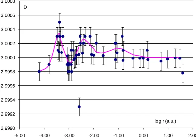
Figure 13 shows the calculation results using this equation defining the parameter D for the objects of the Solar system known by the year of 1990 [27] [28]. As is evident from Figure 13, the amplitude of variation of this parameter increases in a statistically significant manner with a decrease in the distance. The point D = 2.9993 corresponds to the Moon.

The only object falling out of the entire data array for satellites is the Moon (log r = –2.59). As for the plane-tary scale from the Mercury to Neptune, the parameter D = 3 falls within the measurement error.

The author does not assume the responsibility for interpretation of the physical reasons underlying this phe-nomenon. However, since the goal of this work is to formulate a hypothesis verifiable for the origin of life to the extent possible that would fundamentally differ from all the previously proposed hypotheses, we well use the results obtained by analyzing variations in the parameter D to formulate the following hypothesis:

In the vicinity of gravitating masses in the space on the average uniform and isotropic, spherical layers of a fractal space structure are formed, the dimensionality of which is subject to small variations in the neighbor-hood of the integer value D = 3.

Consider the possible consequences of such variation in space dimensionality in the context of the stated problem.

Assuming that the observed variation is not a consequence of an accuracy error (which is actually impossible, because otherwise it would be similarly impossible to observe the variations in DR but only a monotonic drift),

we can postulate that the physical vacuum additionally influences the pattern of satellite motion. Vacuum is among the most mysterious material substances, whose properties are being discussed among theoretical phy-sicists for already several decades. We will take advantage of the current concepts on physical vacuum by vari-ous authors [29]-[31] to try to extract the rational kernels for construction our own view on solution of the prob-lem of the origin of life.

Figure 13. Dependence of the parameter D on the distance of satellite from the central body. The abscissa shows the decimal logarithm of the distance in astronomic units. 2.9990

2.9992 2.9994 2.9996 2.9998 3.0000 3.0002 3.0004 3.0006 3.0008

-5.00 -4.00 -3.00 -2.00 -1.00 0.00 1.00 2.00 D

During the last decade, the terms dark energy and antigravitation [31] have been formulated and almost es-tablished in the scientific worldview. Although the concept of antigravitation was introduced by Einstein as long ago as 1917, it was really comprehended only after analyzing the cosmological observations during several re-cent years. In fact, antigravitation significantly manifests itself in repulsion of galaxies on a scale of five to eight billion light years. Therefore, it is quite evident that it is fundamentally impossible to observe antigravitation by the same methods on planetary scales to say nothing about the scale of Earth. However, the goals of this work do not require this, since the mere fact of antigravitation and its recognition in the scientific community is suffi-cient.

6. Conclusions

From the standpoint of the author, in addition to the standard physiologically necessary conditions for sustaina-ble existence of life, namely, “normal” pressure, temperature, and humidity of environment and the absence of pathogenic physical and chemical factors, polarization of the physical vacuum is a basically important factor for self-organization of molecules into a self-replicating system [29] [30].

The consequence of this is a fractal, i.e., noninteger, space-time dimensionality, which entails nonlinearity of all molecular processes eventually giving rise to a spatiotemporal ordering of the molecular processes that had led to formation of self-replicating informational structures. Note that the noninteger, i.e., fractional, dimensio-nalities of both space and time separately also gave in sum an integer, an invariant of four!

Acknowledgements

The author is grateful to Prof. A.D. Gruzdev, Prof. S.A. Shnoll, Prof. R.G. Khlebopros for fruitful discussions.

References

[1] Gusev, V.A. and Gruzdev, A.D. (2011) Laws of the Evolution of Living and Inanimate Material. The Periodical of the

Problems of the Evolution of the Open Systems, 2, 89-107.

[2] Elin, V.L. (1957) On the Biology of Coliform Bacillus. Microbiology, 26, 17-21. (in Russian)

[3] Kalinenko, V.O. (1957) Reproduction of Heterotrophic Bacteria in Distilled Water. Microbiology, 26, 148-153. (in

Russian)

[4] Gusev, V.A. (2001) On the Source of Energy for Preservation of Viability and Amplification of Heterotrophic

Micro-organisms under Conditions of Substrate Starvation. I. Formulation of Hypothesis. Biophysics, 46, 862-868. (in

Rus-sian)

[5] Gusev, V.A. and Neigel, N.J. (2001) On the Source of Energy for Preservation of Viability and Amplification of

Hete-rotrophic Microorganisms under Conditions of Substrate Starvation. II. Substantiation of Hypothesis. Biophysics, 46,

869-874. (in Russian)

[6] Gusev, V.A. (2001) On the Source of Energy for Preservation of Viability and Amplification of Heterotrophic

Micro-organisms under Conditions of Substrate Starvation. III. Necessary and Sufficient Conditions for MicroMicro-organisms to

Colonize Water Envelopes of Planets. Biophysics, 46, 875-878. (in Russian)

[7] Gusev, V.A. (1992) Evolution of Microbial Cell Population under Complete Substrate Starvation. Evolutionary

Simu-lation and Kinetic. Nauka, Novosibirsk.

[8] Gusev, V.A., Evdokimov, E.V. and Bobrovskaya, N.I. (1992) Deviation from Poisson Distribution in the Series of

Identical E. coli Cell Culture. Biophysics, 7, 733-737.

[9] Gusev, V.A. (2008) Evolutionary Drift, Cooperative Effects, Quasiperiodic Variations, and Biorhythms of Microbial

Communities under Extreme Conditions of Absolute Substrate Starvation. The Periodical of the Problems of the

Evo-lution of the Open Systems, 1, 130-138. (in Russian)

[10] Gusev, V.A. and Schulze-Makuch, D. (2005) Low Frequency Electromagnetic Waves as a Supplemental Energy

Source to Sustain Microbial Growth? Naturwissenschaften, 92, 115-120. http://dx.doi.org/10.1007/s00114-004-0594-9

[11] Gusev, V.A. (2012) Electromagnetic Waves as the Source of Free Energy for the Living Systems. LAP Lambert

Aca-demic Publishing, Saarbrucken, 204.

[12] Chernoshchekov, K.A. and Lepekhin, A.V. (1992) On the Vital Activity of Enterobacteria in the Aqueous Medium in

the Absence of the Sources of Organic Power. Journal of Microbiology, Epidemiology and Immunology, 9, 21-24. (in

Russian)

Biological Objects. Proceeding of SPIE, 3732, 196-201.http://dx.doi.org/10.1117/12.340011

[14] Smirnov, B.M. (1991) Physics of Fractal Clusters. Nauka, Moscow. (in Russian)

[15] Feder, J. (1989) Fractals. Plenum, New York.

[16] Gusev, V. (2001) Living Universe. Palyi, G., Zucchi, C., et al., Eds., Elsevier, Paris, 41-46.

http://www.geocities.com/awjmuller/pdf_files/LivingUniverse.pdf

[17] Gusev, V.A. and Schulze-Makuch, D. (2004) Genetic Code: Lucky Chance or Fundamental Law of Nature? Physics of

Life Reviews, 1, 202-229.http://dx.doi.org/10.1016/j.plrev.2004.11.001

[18] Gusev, V.A. (2005) Arithmetic and Algebra in the Structure of Genetic Code, Logic in the Genome Structure and

Bio-chemical Cycle of Self-Replication of Living Systems. Vestnik VOGiS, 9, 153-161. (in Russian)

[19] Oparin, A.I. (1924) The Origin of Life. Moskovskii rabochii, Moscow. (in Russian)

[20] Strugatskiy, A. and Strugatskiy, B. (1976) Billion Years to the End of the Earth. Znanie-Sila, Moscow, No. 9-12. (in

Russian)

[21] Gusev, V.A. (2002) Chemical Evolution in a Thunderstorm Cloud. Doklady Chemistry, 385, 186-188. (in Russian)

http://dx.doi.org/10.1023/A:1016583017174

[22] Somsikov, V.M. (2006) At the Beginning Physics of Evolution. The Periodical of the Problems of the Evolution of the

Open Systems, 2, 9-17. (in Russian)

[23] Carr, B.J. and Rees, M.Y. (1979) The Anthropic Principle and the Structure of the Physical World. Nature, 278, 605-

612. http://dx.doi.org/10.1038/278605a0

[24] Gorelik, G.E. (1983) Dimensionality of Space. Moscow State University, Moscow. (in Russian)

[25] Ehrenfest, P. (1917) In What Way Does It Become Manifest in the Fundamental Laws of Physics that Space Has Three

Dimensions? Proceedings of the Amsterdam Academy, 20, 200.

[26] Gorelik, G.E. (1982) Why Space Is Three-Dimensional? Nauka, Moscow. (in Russian)

[27] Abalkin, V.K., Ed. (1981) Astronomic Almanac (Constant Part). Nauka, Moscow. (in Russian)

[28] Marov, M.Ya. and Zharkov, V.M., Eds. (1990) The System of Saturn. Mir, Moscow. (in Russian)

[29] Dyatlov, V.L. (1998) Polarization Model of Inhomogeneous Physical Vacuum. Izd. IM SO RAN, Novosibirsk. (in

Russian)

[30] Dmitriev, A.E., Dyatlov, V.L. and Gvozdarev, A.Yu. (2005) Unusual Phenomena in Nature and Inhomogeneous Vacuum.

Izd. BTPU im. Shukshina, Novosibirsk-Gorno-Altaisk-Biisk. (in Russian)