Modelling Devices for Natural Interaction

Modelling Devices for Natural Interaction

Alan Dix

Computing Department, InfoLab21 Lancaster University

Lancaster, UK

Masitah

Ghazali

Devina Ramduny-Ellis

Information Systems Department Computing Department, InfoLab21 Universiti Putra Malaysia, Lancaster University

Malaysia Lancaster, UK

Abstract

We do not interact with systems without first performing some physical action on a physical device. This paper shows how formal notations and formal models can be developed to account for the relationship between the physical devices that we actually press, twist or pull and their effects on systems. We use state diagrams of each but find we have to extend these in order to account for features such as bounce-back, where buttons or other controls are sprung. Critical to all is the fact that we are physical creatures and so formal models have to take into account that physicality.

Keywords: physicality, interaction modelling, affordance, natural interaction, physical devices

1 Introduction

For some years we have been interested in understanding what makes some interactions with physical devices seem ‘natural’ whilst others need to be carefully learnt. Part of this lies in the fact that interacting with ordinary objects in the physical world is natural to us, even as babes we reach out, explored our own hands, touched our mothers’ faces, then played with balls and toys. Many aspects of physical interaction are informed by culture and things we have learnt about the technological world, but much is still common and would be equally natural if a person from two hundred or even two thousand years ago were suddenly transported to the present.

1

Supported by AHRC/EPSRC funded project DEPtH “Designing for Physicality” www.physicality.org

2 _{Email: [email protected]}

3 _{Email: [email protected]} 4

One aspect of our studies has been to try and unpack which properties of physical interaction are essential to make them comprehensible, and which can be relaxed [[GD03,D03,GD05]]. This can then be used to understand how to make digital interactions themselves more natural, and thus inform several forms of design:

• pure digital interaction on a computer screen (although even this requires physical devices, such as the mouse)

• novel tangible interactions where physical objects are endued with digital properties (as found in tangible interaction, and ubiquitous computing)

• more mundane devices such as mobile phones or even electric kettles

A critical method for us has been to analyse in detail ordinary commonly used artefacts such as an electric kettle or mini-disk controller (already looking very dated!). We assume that when such devices appear easy to learn and use the designers have often embodied, either explicitly or implicitly, their own understanding of what makes interaction natural. So by this detailed analysis we gradually mine this, often tacit, experience of successful designers.

In this paper we describe how, as part of this work, we use separate but connected models of physical devices and of their digital effects. By separately modelling these we can discuss the physical aspects of a device and also the extent to which this relates sensibly to the digital aspects. In some ways this is similar to architectural models from Seeheim on [[PH85]] that separate presentation from functionality, but in these the different levels are all principally digital, with only Arch/Slinky making an explicit attempt to discuss physical level of interaction [[U94]]. However, even Arch/Slinky puts physical interaction as an additional (lowest) layer whilst we shall see that physical devices embody aspects of at least dialogue-level interaction.

In the next section we unpack the way in which physical devices relate to their digital effects on a system’s logical state and the kinds of feedback that occur. Section 3 then reviews some critical related work. The bulk of this paper goes step by step through a number of example devices and systems of increasing complexity and builds up ways of describing these in terms of state diagrams and develops a formal model of each. Finally we reflect on the lessons learnt and further work required to obtain a complete model of physical interactions with digital devices.

2 Physical

Devices

and

Feedback

When we use the term physical device in this paper we are using the word slightly differently than is common. We use it to mean the actual physical button, knob or other controls on their own. For example, when a light switch has properties when torn from the wall and unwired – that is the physical device is the switch whether or not it is connected to a light. In the case of a mobile phone think of the phone with its innards removed – you can hold it, press its buttons etc., whether or not you get any digital feedback. Sometimes the term ‘physical device’ would be used for the phone together with its digital functionality, but by separating the two we aim to understand better the relationship between them.

effective feedback was one of Shneiderman’s aspects of direct manipulation [[S83]], one of Nielsen’s heuristics [[NM94]] and a substantial issue in the early formal modelling of interactive systems captured in various forms of observability [[D91]].

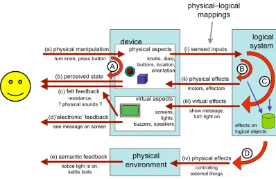
Once we think of the physical device and the digital effects separately, we can look at different ways in which users get feedback for their actions. Consider a mouse button: you feel the button go down, but also see an icon highlight on screen.

Figure 1. Multiple feedback loops

Figure 1 shows some of these feedback loops. Unless the user is implanted with a brain-reading device, all interactions with the machine start with some physical action (a). This could include making sounds, but here we will focus on bodily actions such as turning a knob, pressing a button, dragging a mouse. In many cases this physical action will have an effect on the device: the mouse button goes down, or the knob rotates and this gives rise to the most direct physical feedback loop (A) where you feel the movement (c) or see the effect on the physical device (b).

In order for there to be any digital effect on the underlying logical system the changes effected on the device through the user’s physical actions must be sensed (i). For example, a key press causes an electrical connection detected by the keyboard controller. This may give rise to a very immediate feedback associated with the device; for example, a simulated key click or an indicator light on an on/off switch (ii). In some cases this immediate loop (B) may be indistinguishable from actual physical feedback from the device (e.g. force feedback) in other cases, such as the on/off indicator light, it is clearly not a physical effect, but still proximity in space and immediacy of effect may make it feel like part of the device.

text, for a MP3 player a new track or increased volume. This change to the logical state then often causes a virtual effect (iii) on a visual or audible display; for example an LCD showing the track number (iii). When the user perceives these changes (d) we get a semantic feedback loop (C). In direct manipulation systems the aim is to make this loop so rapid that it feels just like a physical action on the virtual objects.

Finally, some systems affect the physical environment in more radical ways than changing screen content. For example, a washing machine starts to fill with water, or a light goes on. These physical effects (iv) may then be perceived by the user (e) giving additional semantic feedback and so setting up a fourth feedback loop (D).

For the purposes of this paper we will not care much whether the final semantic effect and feedback is virtual (loop (C)) or physical (loop (D)) as it is the physical device that we are most interested in.

3 Related

Work

The most obvious connection to this work is Gibson’s concept of affordances [[G86]]. For a simple physical object, such as a cup, there is no separate logical state and simple affordances are about the physical manipulations that are possible ((a) in Figure 1) and the level to which these are understood by the user: Norman’s ‘real’ and perceived affordances [[N99]]. For a more complex, mediated interface the effect on the logical state becomes critical: the speaker dial affords turning but at another level affords changing the volume. Hartson [[H03]] introduces a rich vocabulary of different kinds of affordances to deal with some of these mediated interactions.

Benford et al.’s SSD framework [[BS03]] deals with this relationship between the physical device and logical state. It considers three aspects of the relationship: sensable – the aspects of the physical device can be sensed or monitored by the system, sensible – the actions that the user might reasonably do to the device, and desirable – the attributes and functionality of the logical system that the user might need to control. This is used to explore the design space and mismatches between the sensible, sensable and desirable may suggest options for re-design. In Figure 1, the sensable aspects correspond to (i), whilst the sensible ones refer to possible actions (‘real’ affordances) of the device (a) that the user might reasonably perform. The desirable part of the framework refers to the internal possibilities of the logical state. Note what is sensible to do with a device depends partly on perceived affordances and partly on the user’s mental model of the device and its associated logical state.

The concept of fluidity, introduced in Dix et al. [[DF04]] and expanded in the work leading to this paper, is focused on the way in which this mapping is naturally related to the physical properties of the device. Whereas the SSD framework is primarily concerned with what it is possible to achieve, fluidity is focused on what is natural to achieve.

feedforward is, rather like Norman’s perceived affordance, about the different ways a device/system can expose its action potential. Critically too, this work, like our own, is interested in what makes interaction natural and brings out particular qualities that impact this: time, location, direction, dynamics, modality and expression.

4 Exposed States and Physical–Logical Mapping

4.1 Example – up/down light switch

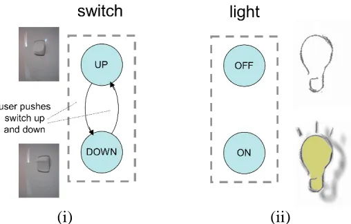
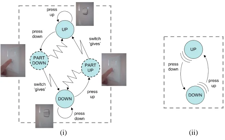
One of the simplest examples of a physical device is a simple on/off light switch. In this case the switch has exactly two states up and down and pressing the switch changes the state (Figure 2.i).

Actually even this is not that simple as the kind of press you give the switch depends on whether it is up and you want to press it down or down and you want to press it up. For most switches you will not even be aware of this difference because it is obvious which way to press the switch … it is obvious which way to press it because the current state of the switch is immediately visible.

Note that the switch has a perceivable up/down state whether or not it is actually connected to a light and whether or not the light works.

The logical system being controlled by the device also has states and figure 2.ii shows these in the case of the light bulb simply on or off. (in fact the light bulb may also be broken, but we are ignoring faults for this discussion).

(i) (ii)

Figure 2. Light switch (i) physical device (ii) logical states

(e.g. external security lighting); in these case the feedback inherent in the device is not just very obvious, but may be the only immediate feedback.

4.2 Formal Model

We can model this kind of behaviour more generically. We denote by UA the set of potential user actions such as ‘push up’; these may be particular to a specific device ‘push button A’ as our environment affects our action possibilities. We use PA to denote the set of perceivable attributes of the world “light is shining”, “switch is up”. The full perceivable state of the world is composed of the different perceivable effects and there may be masking effects if light 1 is on we may not be able to tell that light 2 is on also. However, for simplification we will just assume these are individually identifiable – at least potentially perceivable.

The physical device we model as a simple state transition network: DS – physical states of device

DT DS DS – possible device transitions

In the light switch every transition (only two!) is possible, but in some situations this may not be the case. Hence the physically possible transitions are a subset of all conceivable from–to pairs. Some of these transitions are controlled by user actions:

action: UA DT – n–m partial relation

Note that this relation is n-to-m, that is the same user action may have an effect in several states (with different effect) and a single transition may be caused by several possible user actions (e.g. pressing light switch with left or right hand). In addition neither side is surjective, some physically possible transitions may not be directly controllable by the user (e.g. lifting large weight, pulling out a push-in switch) and some user actions may have no effect in the device in any state (e.g. blowing your nose). However, for exposed-state devices we will normally expect that the states are completely controllable by the user within the physical constraints of the device:

controllable-state action is surjective

Aspects of the user’s state may be perceivable by the user: ddisp: DS PA

And in the case of exposed state each device state is uniquely identifiable by its visible or other perceivable attributes:

exposed-device-state ddisp is injective

Finally the logical system also has states which themselves may be perceivable via the feedback loops C or D.

LS – logical states of system ldisp: LS PA

For any system we can define a map describing which device states and logical states can occur together:

state-mapping: DS LS

The precise nature of this mapping depends on the operation of the system. In some cases like the light switch this is a one-to-one mapping between the physical device and logical states and this is precisely what we mean by exposed state.

Note also that user actions such as pressing a button are not simply ‘events’, but are protracted over time and vary in force. An additional way in which the user gets feedback on the state of the device and appropriate actions is by ‘trying out’ an action, often unconsciously, and if there is a small give in the device continuing the action and increasing pressure until the user action causes a change in state of the device.

The importance of this kind of effects are hinted at by Gaver in 1991, when he introduced sequential affordances [[G91]], and are clearly part of design practice, but not discussed more explicitly to our knowledge in the HCI literature. We do not explore this fully in this paper, but some aspects that are critical to the argument.

5 Bounce Back Buttons

5.1 Example – push on/off switch

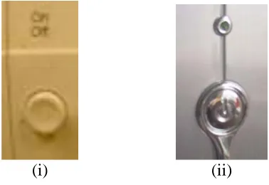
A more complex behaviour occurs with bounce-back buttons or other devices where there is some form of unstable state (pressed in, twisted) where you need to maintain constant pressure to maintain the state. Figure 3.i shows a typical example of a computer on/off switch. One press and release turns it on, a second turns it off.

(i) (ii)

Figure 3. (i) On/Off control with bounce back – is it on or off now? (ii) On/Off button with indicator light

Note, following the discussion at the end of the last section, that the user action here, – pressing the button – is not discrete, but involves pressing until it ‘gives’ then releasing. While you maintain pressure the button stays in, it is when you release that it comes out again. However, the button comes out not because you pull it out with your release of pressure, but because it is internally sprung – the bounce-back.

Bounce-back buttons are found everywhere, from keyboards, to mice to television sets. They typically do not expose the state of the underlying system as there is just one stable state of the physical device and it is the history of dynamic interactions with it that is important (on or off, what channel). The temporary unstable states of the device are maintained by the continued pressure so are distinguishable, while they are maintained, but the physical device itself does not maintain a record of its interaction in the way a rocker switch does.

D) is sufficient – for example, switching channels on a television set. However, even where there is semantic feedback this may be ambiguous (switching channels during advertisement break) or delayed (the period while a computer starts to boot, but is not yet showing things on screen). In such cases supplemental feedback (loop B) close to the device is often used, such as a power light on or near the switch (Fig 3.ii).

Where the device does not have an intrinsic obvious tactile or audible feedback (e.g., click of the switch or feeing of ‘give’ as it goes in) then supplemental loop (B) feedback may be given for the transitions as well as the states. Simulated key clicks or other sounds are common, but also, more occasionally, simulated tactile feedback can be used, as in the BMW iDrive.

From a design consideration indirect feedback, whilst less effective, is useful in situations where the complexity of the underlying system exceeds the potential states of the device. In particular, bounce-back controls are used precisely (but not only) when we wish to transform user’s continuous actions into discrete events.

5.2 Formal Model

We can inherit much of the same machinery from simple exposed-state devices. However, in addition to transitions controlled by the user we have bounce-back transitions. We label them Z (after Zebedee and the fact that Z and S are used for left- and right-handed helices). In the example here there is only one action leading to the states and thus it is clear what kind of user tension needs to be released in order for the bounce-back to happen. Sometimes (and we will see an example later) there is more than one tension simultaneously for a state, so we need to label the bounce-backs by the kind of release of tension (in terms of user action) that is being released.

Z: UA DT

The states that are the subject of bounce-back transitions are transitory states for that user action:

a UA transitory-states(a) { d DS, st. (d,d’) Z(a) }

Furthermore a transitory state for a user action cannot be the source of the same user-controlled transition and must have been reached by that user action:

a UA

transitory-states(a) dom( action( a ) ) = {} transitory-states(a) range( action( a ) )

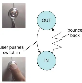
Figure 4 shows the example of the computer switch with the bounce-back transition shown as a zig-zag line (spring) and the transitory state (IN) dotted.

While exposed state devices can have a one-to-one mapping between logical sates and physical states, here the relationship is based on the events. Formally we define this first by associating events from a set Ev with physical state transitions:

trigger: DT Ev

This mapping may be partial as not every transition will cause an event and the μ

Figure 4. States of bounce-back button

These events then cause transitions in the logical system: doit: Ev LS LS

Figure 5 shows the physical device STN annotated with an event (a) and the effect of the event on the logical state (computer power). Note that in this example (and it is common!) there is no reason why the system could not have been designed with exposed state, for example a button that stays depressed an requires an extra push to release it. This design choice is often motivated by the aim to have a smooth surface although in the example in Figure 3.ii the switch is part of an embellishment anyway, so even this aesthetic reason seems to be absent.

(i) (ii)

Figure 5. (i) physical states changes trigger event (a) (ii) logical state changes based on events

5.3 Recapitulation – the exposed state switch

pushed down. If you release before putting sufficient pressure on it snaps back to UP, but if the pressure is sufficient the switch yields and goes to the new state.

This yielding is rather like bounce back in that once the critical point is reached the device just goes of its own accord. However, we have drawn it slightly different (less off a spring and more of lightening bolt in order to emphasise that this is going ‘with’ the user’s action and it is the point at which the ‘commitment’ occurs.

(i) (ii)

Figure 6. Capturing initial pressure on exposed state switch (i) detailed model using bounce-back

(ii) more convenient shorthand

Note that in figure 6.i a transition is included for “press up” in the Up state which simply leaves the switch in the UP state. This distinguishes ‘press down’, for which there is a little give with a small pressure, from ‘press up’, for which there is no give. Thus we can begin to capture some of the nature of Gaver’s sequential affordances.

In fact to model this completely we would need to include degrees of pressure and the fact that there is no just one half pressed-down state, but a whole series requiring increasing pressure. This is not captured by a finite state diagram or description and would require a full status–event description as we are talking here about interstitial behaviour (the interaction between events) and status–status mapping (more pressed = more down) [[DA96]]. This is also reminiscent of Buxton’s three-state model for pointing devices, where the degree of finger pressure is one of the critical distinctions between abstract states [[B90]].

typically fully electronic ones. Formally we can capture this by a simple ‘has-give’ predicate over user actions in particular states.

6. Time-dependent devices

6.1 Example – Track/Volume Selector

Our next level of complexity are devices such as keyboards with auto-repeat or, tuning controls on car radios where things happen depending on how long you have been in a state. Figure 7.i shows a mini-disk controller. The knob at the end can be pulled in or out turned to the left or right. Figure 7.ii shows this physical state transition diagram of the device. This would probably be better described using two STNs one for in-out and one for left-right, but as they are coupled in a single control we are showing all the transitions to give an idea of the total complexity of even such a simple thing as one knob!

(i) (ii)

Figure 7. (i) minidisk controller (ii) device states

Whether the knob is pulled in or out determines whether it is affecting the volume or track selection and the amount of time it is pushed to the left or right moves the volume/track selection up or down. The former is a simple mode effect … and a tension mode carries its own feedback, so is a god design feature. However, we shall focus on the left-right twists and their time behaviour.

user is aware that they are holding the device in tension – while the exact times when events are triggered is not totally under the user’s control (unless they have a millisecond clock in their heads!), still the fact that it is being held is readily apparent.

(i) (ii)

Figure 8. minidisk (i) time augmented device (ii) logical states

6.2 Formal Model

Notice that everything in figure 7.ii, with the exception of CENTRE-IN, is a tension state. However, there are actually two kinds of tension demonstrating why we needed to label transitory states and bounce-backs by user actions in section 4.2.

In Figure 8.i we draw the timed events as if they were transitions, however we model them simply as an aspect of the state. This is because for the user the system does not make little transitions to the same state, it simply stays in the tension state. There may also be real timed transitions, but these are more often in response to things happening in the logical state, which we discuss in the next section. So all we need to do is say in which state and how often and frequently the timed events occur.

time-trigger: DS x Time x Kind Ev

Here Time is as in gap between moments rather than time on the clock, and Kind is either PERIODIC or SINGLE

Note that this is another example of interstitial behaviour and shows again that a more fine-grained model would need to use a full status–event description. Also to express precisely the semantics of time-trigger we need to use a real-time model.

7. Controlled state and compliant interaction

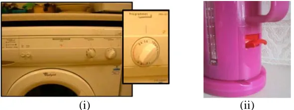
7.1 Example – Washing Machine and Electric Kettle

Finally we come to devices where the state of the physical device is affected by the underlying logical system as well as vice versa. Consider a washing machine control knob that sets the programme (Figure 9.i) or an electric kettle switch (Figure 9.ii). In each case the user can control the device: twisting the knob to set the programme or pushing up or down the kettle switch to turn on an off the kettle. However, in addition the underlying logical system can also effect the physical device. In the case of the washing machine as the clothes are washed the dial usually moves round to act as a display of the current state of the programme. In the case of the kettle, when the water boil many kettles both switch themselves off and at the same time release the switch. We say that this kind of device has controlled state.

In fact both systems also exhibit compliant interaction [[GD03]] where the system control of the physical device operates in a compatible way to the user control: with the kettle the user can turn the switch off or the system can. Of course there are usually limits to compliant interaction: the kettle does not turn itself on and the user turning the knob to the end of the wash cycle does not magically wash the clothes!

(i) (ii)

Figure 9. compliant interaction (i) washing machine knob (ii) kettle switch

Figure 10 shows the state diagram for the kettle switch and also the state of the power and water. Strictly thee are two sub-systems in the kettle the power (ON/OFF) influencing the water temperature (continuous scale), but for simplicity we have shown the water state as simply boiling vs. not boiling and only as sub-states of the POWER-ON state. The arrows between the device and logical state show that there is an exposed state for the electrical power system. The little lightening arrow from the water’s BOILING state shows that simply being in the state triggers the system action ‘system down’. Like user actions in the physical world this is protracted and lasts as long as the kettle is boiling, it is not simply an event at the moment boiling is first sensed. This possibility of an autonomous action is shown by the dashed transition on the state diagram for the physical switch.

switch up (usually simply releasing a catch) so it is possible to boil the kettle when dry. You could imagine a kettle design where the power was switch off by the system when the water was boiling irrespective of whether the user allows the switch to go down, in this case we would have similar device states, but a different logical state transitions and no exposed state mapping.

(i) (ii)

Figure 10. electric kettle (i) kettle switch (ii) power and water

7.2 Formal Model

To deal with these kinds of devices we need to add a set of system actions SA and have a mapping that says which systems actions are triggered by which logical stats:

sys-trigger: LS set(SA)

These system actions will then have their effect on device state transitions just like user actions:

sys-action: SA DT – n–m partial relation

Just like user actions it is possible that a single system action may gave different effects in different device states and that several system actions might be possible in a single device state. However, when it is an exposed state system, like the kettle, it is likely that the system actions are very specific for a particular state. Indeed if there is a state-mapping, then there should be some consistency between the system state(s) that correspond to a device state and the system actions pertaining to each:

a SA, s LS

a sys-trigger(s) d DS st. (d,s) state_mapping a SA, d DS

d dom(sys-action(s)) s LS st. (d,s) state_mapping The first of these says that is a logical state can trigger a system action then at least one of the device states consistent with that logical state must take account of that system action. The second says the converse that if a device state can be affected by a system action then it must be possible for one of the logical states consistent with that device states to generate the action.

being ignored. This may be an intended effect of the combination, but certainly merits checking.

Finally for this example, the logical system state itself was more complex. We had two subsystems power and water, which we represent by abstraction functions:

power: LS PowerState water: LS WaterState

When the two sub-systems are orthogonal (any combination of sub-system states is possible) and between them completely define the logical state, then LS is simply the Cartesian product of the sub-system states and the abstraction functions simply the component mappings.

Given such sub-system mappings we can define what it means for the system to exhibit exposed state relative to a sub-system:

exposed-state wrt. power (power state-mapping) is one-to-one

Discussion

We have used a number of examples to show different ways in which the physical states of a device can interact with the logical states of the system. These have reinforced the importance of distinguishing the two and being able to talk about the sometimes quite subtle differences between what might appear to be similar controls.

Each example has dealt with a different property that we have introduced in previous work: exposed state, hidden state, bounce-back, controlled state and compliant interaction. For each of these we have (i) discussed examples informally, then (ii) expressed the examples using parallel state transition networks for the physical and logical states and (iii) given these semantics using a formal model. We have introduced the formal model piecewise as each property requires additional elements in the model.

For practical design the variants of STNs would seem more appropriate than the model, although the later gives the former a more precise semantics. The simpler examples and the relationship between the physical and logical STNs could be dealt with using standard notations and certainly could be translated into state-charts or similar notations. However, as we looked at more complex properties such as bounce-back we had to extend standard state-transition networks to represent the additional effects. This exposes design issues such then appropriate use of tension states.

References

[1} [[BS03]] Benford, S., Schnadelbach, H., Koleva B., Gaver, B., Schmidt, A., Boucher, A., Steed, A., Anastasi, R., Greenhalgh, C., Rodden, T., and Gellersen, H. Sensible, Sensable and Desirable: A Framework for Designing Physical Interfaces. Technical Report Equator-03-003, Equator, 2003 (www.equator.ac.uk)

[2} [[B90]] Buxton, W. A Three-State Model of Graphical Input. In D. Diaper et al. (Eds), Human-Computer Interaction - INTERACT '90. Amsterdam: Elsevier Science Publishers B.V. (North-Holland), (1990), 449-456.

[3} [[D91]] Dix, A. Formal Methods for Interactive Systems. Academic Press, 1991.

[4} [[DA96]] Dix, A. and Abowd, G. Modelling status and event behaviour of interactive systems. Software Engineering Journal, 11:6 (1996), 334-346.

[5} [[D03]] Dix, A. Getting Physical. keynote at OZCHI 2003, Brisbane, Australia, 26-28 Nov 2003

[6} [[DF04]] Dix, A., Finlay J. Abowd, G. and Beale R. Human-Computer Interaction. Third Edition. Prentice Hall, 2004.

[7} [[G91]] Gaver, W. Technology affordances. In Proc. of CHI '91. ACM Press, (1991),79-84.

[8} [[GD03]] Ghazali, M. and Dix, A. Aladdin's lamp: understanding new from old. In 1st UK-UbiNet Workshop, 25-26th September 2003, Imperial College London

[9} [[GD05]] Ghazali, M. and Dix, A. Visceral Interaction Proceedings of the 10th British HCI conference, Vol 2, September 5-9, Edinburgh. (2005), 68-72

[10}[[G86]] Gibson, J. The Ecological Approach to Visual Perception. Houghton Mifflin Company. USA, 1986.

[11}[[H03]] Hartson, H. R.. Cognitive, physical, sensory, and functional affordances in interaction design. Behaviour & Information Technology 22:5 (2003) , 315–338.

[12}[[NM94]] Nielsen, J.; Mack, R.L. Usability Inspection Methods. John Wiley & Sons, New York, NY, 1994.

[13}[[N99]] Norman, D. Affordance, conventions, and design. Interactions 6(3): ACM Press: NY, (1999), 38-43

[14}[[PH85]] Pfaff, G., and Hagen. P., (Eds.). Seeheim Workshop on User Interface Management Systems, Springer-Verlag, Berlin, 1985.

[15}[[S83]] Shneiderman, B. (1983). Direct manipulation: a step beyond programming languages. IEEE Computer 16(8) (August 1983), 57-69.

[16} [[WD04]] Wensveen, S. A. G., Djajadiningrat, J. P., and Overbeeke, C. J. 2004. Interaction Frogger: A Design Framework to Couple Action and Function. In: Proceedings of the DIS’04 Cambridge, USA.