http://dx.doi.org/10.4236/ojs.2014.43016
On Minimizing the Standard Error
of the Slope in Simple Linear
Regression
Steven M. Crunk, Xinh Huynh
Department of Mathematics and Statistics, San Jose State University, San Jose, USA Email: [email protected], [email protected]
Received 8 February 2014; revised 8 March 2014; accepted 15 March 2014
Copyright © 2014 by authors and Scientific Research Publishing Inc.
This work is licensed under the Creative Commons Attribution International License (CC BY). http://creativecommons.org/licenses/by/4.0/
Abstract
A common homework problem in texts covering calculus-based simple linear regression is to find a set of values of the independent variable which minimize the standard error of the estimated slope. All discussions the authors have heard regarding this problem, as well as all texts with which the authors of this paper are familiar and which include this problem, provide no solution, a partial solution, or an outline of a solution without theoretical proof and the provided solution is incorrect. Going back to first principles we provide the complete correct solution to this problem.
Keywords
Minimization; Variance; Coefficient; Beliefs about Statistics; Statistical Literacy
1. Introduction
A homework question, occurring in several oft cited best-selling introductory texts covering calculus-based sim-ple linear regression, goes something like this:
Suppose we are to collect data and fit a straight-line simple linear regression, yi=β0+β1xi+i. The errors
are assumed to have mean zero, unknown variance σ2 and to be uncorrelated with one another. Further sup-pose that in this designed experiment, the region of interest for x is A≤ ≤x B, A<B, and that the primary goal is to make the standard error of the estimate of the slope as small as possible. For a given sample size n, at what values of the independent variable should the observations be taken? That is, how should x x1, 2,,xn be
chosen so as to minimize the standard error of the estimate of β1.
(
)(
)
(
)
1 1 2 1 ˆ n i i i n i ix x y y
x x β = = − − = −
∑
∑
which has standard deviation
( )
(
)
2 1 2 1 ˆ . n i i V x x σ β = = −∑
The estimated standard deviation, or standard error, is found by replacing σ2 by its estimate
(
)
22 1 ˆ ˆ . 2 n i i i y y n σ = − = −
∑
The error variance σ2 is an unknown constant and its estimator cannot be formed until data are collected. Thus in the case of either the theoretical standard deviation or the estimated standard error, the numerator under the radical is unknown and not under the control of the experimenter in the question. Consequently the minimi-zation of the standard deviation or the standard error is achieved by maximizing the quantity
(
)
2 1 SXX , n i i x x = =∑
−the corrected sum of squares of the x’s.
Many texts which include this problem provide no solution. Every discussion that the authors have heard dis-cussed or seen in a solutions manual suggests, without proof, that in order to maximize SXX if n is even, half of the observations should be taken at A and half at B. Many texts that include a solution ignore the possibility that n is odd, even though no condition on n was provided in the question. When a solution is provided for n odd, every solution we have seen suggested without proof that
(
n−1 2)
observations should be taken at each of A and B with the remaining single observation being taken half way between these values, at(
A B+)
2. That this solution is incorrect which can be seen with a simple example where n=3. The result using the “usual” solution outlined above is to take x1=A, x2 =B, and x3=(
A B+)
2 from whence x=(
A B+)
2 and(
)
2
SXX= B−A 2. Alternatively, if we take x1=x2=A and x3=B, we have x=
(
2A B+)
3 and(
)
2
SXX=2 B−A 3 which are larger than the value obtained using the “usual” solution, showing that the usual solution is not correct. We suppose that the desire for symmetry led to the belief in the incorrect solution; however symmetry has not been neither mentioned nor required for the problem under discussion.
In the sequel we show that for n even, the “usual” solution of choosing half of the observations to be taken at A and the other half to be taken at B is correct. For n odd we show that in order to minimize the standard error,
(
n+1 2)
observations should be taken at one end of the interval (either at A or at B) and the remaining(
n−1 2)
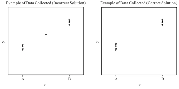
observations should be taken at the other end of the interval. An example of this result is given in Figure 1. Throughout we will assume that the sample size n is a given constant.2. The Objective Function; Sum of Squares
Our goal is to find the set of xi which maximize(
)
2 2 21 1 1
1
SXX .
n n n
j j j
j j j
x x x x
n = = = = − = −
∑
∑
∑
Since the xi are continuous variables (not in the statistical sense but rather in the algebraic sense) on the
in-terval
[
A B,]
, we may use techniques of calculus in order to find the values that maximize this function (see, e.g., [2]). We have1
SXX 2
2 2 2 .
n
i j i
j i
x x x x i
x n =
∂
= − = − ∀
Figure 1. The graphs above represent n (an odd number) data points collected according to two plans for minimizing the standard error of the slope in simple linear regression. The figure on the left represents the common but incorrect solution whereby one observation is taken in the middle of the interval. In the graph to the right, the number of observations taken at either end of the interval differ by one. Although lacking symmetry, this is the correct solution for minimizing the standard error of the slope.
Setting this equal to zero we have xi= ∀x i being stationary points. Of course our variables exist on a
closed interval so we must also investigate the endpoints. As a result it must be true that xi∈
{
A x B, ,}
∀i. If xi= ∀x i then SXX = 0, which is the smallest possible value of SXX, i.e., choosing xi= ∀x i leads to aminimum rather than a maximum. The same is true if observations are taken either all at A or all at B. We would then say it is obvious that at least one observation must be taken at A and at least one observation must be taken at B, but authors saying “it is obvious that...” is what led to this note in the first place. Consider the case where some observations are taken at x=A and the rest at x=x distinct from A; this is a contradiction as the mean would then not be at x . Similarly, it is impossible to have some observations at B and the rest at x. Accor-dingly it must be true that at least one observation must be taken at each of A and B.
Let n1 be the number of observations taken at A, n2 be the number of observations taken at x, and n3 be
the number of observations taken at B. From the argument in the previous paragraph we have ni≥1 for
1, 3
i= , n2≥0, all integers, and n1+n2+n3=n, a given constant. Then x=
(
n A n x1 + 2 +n B3) (
n1+ +n2 n3)
,the simplification of which leads to x=
(
n A n B1 + 3) (
n1+n3)
. Consequently, substituting these values, we have(
)
(
)
2
2 1 3
1 1 1 3
2 2 2
1 3 1 3 1 3
1 2 3
1 3 1 3 1 3
2 1 3
1 3
SXX
.
n n
i i
i i
n A n B
x x x
n n
n A n B n A n B n A n B
n A n x n B
n n n n n n
n n B A
n n
= =
+
= − = − +
+ + +
= − + − + −
+ + +
− =
+
∑
∑
The quantity
(
B−A)
is an arbitrary non-negative constant. Some texts give as their example A= −1 and1
B= , some give A=0 and B=1, and still other books use other choices for these given constants. The choice of A and B, as seen in the final formula for SXX, have no bearing on the solutions for n1, n2 and n3
which maximize SXX. Thus we shall simply attempt to find parameters n1, n2 and n3 that maximize
(
1, 2, 3)
1 3(
1 3)
f n n n =n n n +n with the constraints imposed previously that n1, n2 and n3 are non-negative
integers, n1, n3≥1, and n1+n2+n3=n, a known/given constant.
3. Optimization
Possi-bilities considered by the authors include the following: taking the variables of interest to be continuous and maximizing the function through the use of calculus, hoping for integer values which would then be the optimal solution [3]; using integer programming [4]; and other possibilities. However, it seems that a simple algebraic manipulation may be the most elegant solution.
Let
(
1, 2, 3)
1(
1, 2, 3) (
1 3) (
1 3)
1 3 1 1.g n n n = f n n n = n +n n n = n + n
Thus maximizing f n n n
(
1, 2, 3)
is equivalent to minimizing g n n n(
1, 2, 3)
. We now show that n2 must beze-ro. Assume that
(
n1,0,n2,0,n3,0)
is an ordered triple which meets the constraints and which minimizes(
1, 2, 3)
g n n n with n2,0>0. Let n1,1=n1,0+n2,0, n2,1=0, and n3,1=n3,0. Then the ordered triple
(
n1,1,n2,1,n3,1)
also satisfies the constraints, and furthermore
(
1,1, 2,1, 3,1)
1 3,1 1 1,1 1 3,0 1 1,0(
1,0, 2,0, 3,0)
,g n n n = n + n < n + n =g n n n
which is a contradiction to the assumption that g n
(
1,0,n2,0,n3,0)
minimizes g n n n(
1, 2, 3)
, hence n2 =0.Now one of our constraints reduces to n1+n3=n, and maximizing f n n n
(
1, 2, 3)
=n n1 3(
n1+n3)
reduces tomaximizing
(
1, 3)
1 3(
1 3)
1 3 1 3 1(
1)
.h n n =n n n +n =n n n∝n n =n n n−
This last is simply a parabola which we need to maximize over n1∈
{
1, 2,,n−1}
. To find the maximum,treat the parabola as a function of a continuous variable z. The maximum occurs when ∂z n
(
−z)
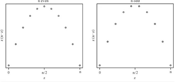
∂ = −z n 2z=0, that is, when z=n 2. As n is integer valued, for n even this implies n1=n 2 gives the maximum value,while for n odd either of the two points surrounding n 2,
(
n−1 2)
or(
n+1 2)
, gives the same maximum value. Figure 2 graphically demonstrates this result. The contradiction in the previous paragraph gives n2 =0and this with the original constraint that n1+n2+n3=n, a known/given constant, gives the value of n3.
4. Conclusions
For the common homework problem appearing in approximately half of the texts covering calculus-based sim-ple linear regression with which the authors are familiar, and which was posed at the beginning of this paper, we have shown that if n is even, the oft given solution to choose half of the points at which to take observations at either end of the interval is correct. However, for odd n we have shown that the only previously given solution to place one point in the center of the interval and half of the remaining points at each end of the interval is in-correct, and that the correct solution is to choose nearly half, either
(
n−1 2)
or(
n+1 2)
, at one end of the interval and the remaining points at the opposite end of the interval.Figure 2.When n is even, the maximum of the objective function occurs at n 2. When n is odd,
[image:4.595.129.500.519.693.2]We part with the common caveat that this oft given textbook problem is of little use in most realistic applica-tions unless it is known that the true relaapplica-tionship among the data is linear, as the solution affords us no opportu-nity to check this assumption with the observed data. However, the authors would submit that there is a differ-ence between being “useless in practical situations” and “understanding something fundamental about simple linear regression”. We believe that it is important for a student to understand the theory underlying simple linear regression, and this importance is supported by the inclusion of the problem in a large number of highly cited and best-selling texts. Unfortunately, many of these texts provide no solution, some provide a partial solution and others provide an incorrect solution. No texts with which we are familiar, nor their solutions manuals, pro-vide a complete and correct solution. This common textbook problem affords the student the opportunity to un-derstand what drives the variance of the parameter estimate, and as such deserves a correct solution.
Acknowledgements
The authors wish to thank Dr. Ho Kuen Ng for a useful discussion on optimization.
References
[1] Weisberg, S. (2005) Applied Linear Regression. 3rd Edition, John Wiley & Sons, Inc., Hoboken. http://dx.doi.org/10.1002/0471704091
[2] Stewart, J. (2011) Calculus. 7th Edition, Thomson Brooks/Cole, Belmont.
[3] Greenberg,H. (1971) Integer Programming. Academic Press, New York.