Munich Personal RePEc Archive
A Theory of Attribution
Feldman, Barry
Prism Analytics
14 March 2007
A Theory of Attribution
Barry E. Feldman
∗May 29, 2007 Version 1.1
abstract
Attribution of economic joint effects is achieved with a random order model of their relative importance. Random order consistency and ele-mentary axioms uniquely identify linear and proportional marginal attri-bution. These are the Shapley (1953) and proportional (Feldman (1999, 2002) and Ortmann (2000)) values of the dual of the implied cooper-ative game. Random order consistency does not use a reduced game. Restricted potentials facilitate identification of proportional value deriva-tives and coalition formation results. Attributions of econometric model performance, using data from Fair (1978), show stability across models. Proportional marginal attribution (PMA) is found to correctly identify factor relative importance and to have a role in model construction. A portfolio attribution example illuminates basic issues regarding utility at-tribution and demonstrates investment applications. PMA is also shown to mitigate concerns (e.g., Thomas (1977)) regarding strategic behavior induced by linear cost attribution.
JEL Classifications: C10, C52, C71, D00, G11, M31 and M41.
Keywords: Attribution, coalition formation, consistency, cost allocation, joint costs, joint effects, proportional value, random order model, relative importance, restricted potential, Shapley value and variance decomposi-tion.
∗Prism Analytics (barry@prismanalytics.com), Russell Investment Group (bfeldman@russell .com) and DePaul University (bfeldma2@depaul.edu). Thanks for comments to Pradeep Dubey, David K. Levine, Herv´e Moulin and an anonymous referee. Questions and comments welcome.
c
What is the relative importance of factors influencing teenage pregnancy or global warming? How should corporate costs or profits be allocated? And what is the relative importance of assets in an investment portfolio?
This paper presents an economic theory of attribution capable of addressing these questions that is based on the general question: “What is the probability that any order of model factors is correctly ordered by their relative importance?” Elemen-tary axioms identify two probability distributions over factor orders. In proportional marginal attribution(P M A), a factor’s expected contribution share is equal the prob-ability it is most important. In linear attribution (LA) all orders are equally likely.
This work is based on and contributes to cooperative game theory, a mathematical approach to the study of bargaining. Cooperative game theory provides models for the representation of the joint effects inherent in bargaining and methods for their attribution. The simplest n-person bargaining game provides a sturdy but limited model of bargaining, yet a perfect structure for the attribution problems studied here. von Neumann (1928/1952) first defines then-person cooperative game. The Shap-ley (1953) value is today the central solution concept. A versatile axiomatically de-fined mathematical structure, it is also the equilibrium outcome of noncooperative bargaining games such as Gull (1988) and Hart and Mas-Colell (1996). It and its gen-eralization to games with a continuum of players, the Aumann-Shapley (1974) value, have been applied to diverse problems, including cost allocation (e.g., Shubik (1962) and Young (1985)), general equilibrium (e.g., Shapley (1964)), and price setting (e.g., Billera and Heath (1982)). Roth (1988) and Hart (2006) provide reviews.
Shapley (1953) shows his value represents the expected marginal contributions of players to a growing coalition when all orders of “arrival” are equally likely. Weber (1988) characterizes the set of all linear random order values. A significant literature has developed (e.g., Khmelnitskya (1999) and Segal (2003)). Linearity, however, prevents the worths of coalitions from influencing the random order arrival process.
Consistency in cooperative games has been based on special games that “reduce” players from an initial game. If a solution concept is consistent, allocations to the remaining players are unchanged. Hart and Mas-Colell (1988) define a reduced game and use it to characterize the Shapley value with consistency. Feldman (1999, 2002) shows parallel results for the proportional value using the same reduced game.
Random order consistency requires that an inert player or factor, one having no joint effects with others, not disturb the probabilities of suborders in which it is not included. The random order approach to consistency does not require a reduced game. This facilitates practical application. Random order consistency is shown to provide a simple and powerful expectations-based approach to cooperative value.
order process influenced by coalitional worths and that it is the equilibrium outcome of a noncooperative bargaining game where players’ probabilities of proposing are proportional to their expected payoff. Khmelnitskya and Driessen (2001) and Calvo and Driessen (2003) study generalizations.
Section 1 of this paper presents a microeconomic model of relative importance based on set marginal contributions in a random order model. Random order consis-tency and other axioms are used to directly identify a probability distribution over orders. The Shapley and proportional values are identified in a common framework, without assuming linearity or proportionality, though the change of a single axiom.
Section 2 defines restricted potentials and obtains proportional value derivatives and coalition formation results. The proportional value is shown not converse mono-tonic. A family of values including the Shapley and proportional values is shown.
* * *
Attribution involves a single monotonic utility function. Players in the corresponding bargaining problem must be assumed to have identical linear utility functions. In attribution, factors and factor sets replace players and coalitions. The worth of a factor set is based on the utility resulting from the presence of its factors or the restriction of utility maximization to the variation of its factors. Three examples demonstrate the potential of this theory of attribution.
Statistical tests ignore joint effects by design. Linear attribution of OLS R2 as
a measure of relative importance is proposed by Hoffman (1960), Lindeman, et al. (1980), Kruskal (1987) and Chevan and Sutherland (1991). McNally (2000) initiates its use in ecology studies. Soofi,et al. (2000) develop a model of linear attribution in categorical analysis. Linear attribution of model R2 allows a factor to appear impor-tant due only to correlations with factors in the true model. Feldman (2005a) first proposes an exclusion axiom which requires that such a factor receive zero attribu-tion share, and with other axioms, characterizes proporattribu-tional marginal attribuattribu-tion of model R2 (there called proportional marginal variance decomposition or PMVD).
Gr¨omping (2006, 2007) provides attribution tools and studies OLS LA and PMA. Section 3 studies econometric attribution. The model objective function is con-sidered to be the utility function of an analyst. Random order consistency is found compatible with econometric attribution. Attributions are found stable and compa-rable across a variety models based on data from Fair (1977). PMA identifies factor relative importance and model relationships missed by joint significance tests.
Section 5 considers cost allocation as an attribution problem. Random order consistency is found to be an appropriate axiom for cost attribution. An example illustrates the relative vulnerability of LA to strategic definition of cost centers.
The conclusion summarizes, compares random order and reduced game consis-tency and considers the common assumption that proportional solutions are transla-tion dependent in the light of results of developed here. Extended proofs follow.
1
Basic results
1.1
General framework
Transferrable utility(TU) games represent theworthof a coalition by a single number. Let N = {1,2, . . . , n} be the players or factors. A standard TU game v is a map
v : 2N → R
+∪0 from all S ⊆ N to the nonnegative real numbers, with v(∅) ≡ 0.
The S⊆N are coalitionsorfactor sets. Let ¯i={i} and ¯1¯2 ={1,2}. Set subtraction of ¯i fromS is written S\¯i. Games are assumed weakly monotonic: v(S∪¯i)≥v(S). In an attribution problem, v(S) is the expected utility of a single decision maker. IfS represents binary characteristics, thenv(S) is the utility resulting from the joint presence of the factors.1 Factor set S may instead provide the decision maker with
decision space ∆S, withσS ∈∆S being a possible choice. Thenv(S) is the maximum
v(S) = max
σS∈∆S
U(σS)−U(∅), (1)
where the null utility U(∅) represents the utility obtained when there are no opti-mization choices. The null utility is the basis point of Feldman (2005b). It is clearly needed with exponential and other utility functions that can generate negative utility. Its importance in other circumstances will become apparent.
The weak monotonicity of v corresponds to the assumption that maximization over a greater number of factors cannot result in a decline in expected utility.
Thedual gametovrepresents the marginal contributions of all coalitions or factor sets. The dual worth w(S) is v(N) minus the worth of the complement of S:
w(S) =v(N)−v(N \S). (2)
1.2
The random order model
Attribution is based on a random order model of relative importance. A discrete marginality replaces the more typical economic focus on continuous marginal condi-tions. In this model factors “arrive,” one at time, to join a growing factor set. Factors
1
Amonotonic cover game, wherev∗
could be indexed by arrival order. However, due to the central role of joint marginal contributions, it is simpler to consider the “last to arrive” as the first in an order. The last to arrive can instead be thought of as “first to leave.”
Anorderr= (r1, r2, . . . , rn) is a permutation of the factors (or players) ofN. The
set of all orders of N is R(N). Define Sr
k = {r1, . . . , rk} to be the set (coalition) of
the first k factors (players) in the order r. These are the last k factors to arrive in order r. If S has k factors, S is included in r, written S ∈ r, if and only if S =Sr
k.
Thus w(Sr
i) is the joint marginal contribution of the last i factors to enter. Let r(i)
be the position of i in order r, so that rr(i) =i. When factors are ordered according
to relative importance, r1 isleast important and rn is most important.
LetrS be an order of the factors of a setS(N and consider anr∈ R(N). Assume that for any iand j inS such thatrS(i)> rS(j), it is also true thatr(i)> r(j). The
order of the factors in rS is preserved in r, so rS is a suborder of r, written rS ⊂ r.
Also,r is a superorder of rS, written r⊃rS.
Let mP(r) be an n-vector of positional marginal contributions defined by r.
Ele-ment i, mP
i (r), represents the marginal contribution of the factor in position i in r.
This quantity is defined as follows with respect to the dual game:
mPi (r) =w(Sir)−w(Si−r 1), i= 1,2, . . . , n, (3)
whereSr
0 =∅andw(∅) = 0. LetmS(r) be then-vector ofset marginalcontributions:
mSi(r) =w(Sir) =v(N)−v(N \Sir(r)), i= 1,2, . . . , n. (4)
The probability p(r) that any order r ∈ R(N) is the realized order of arrivals is defined by a likelihood function L(r) with L(r)≥0 for all r:
p(r∗) = L(r∗)
X
r∈R(N)
L(r). (5)
The expected utility contribution of factor i with respect to distribution p is then
φi(v) = Ep[mPr(i)(r)] =
X
r∈R(N)
p(r)mPr(i)(r). (6)
1.3
Axioms and the fundamental theorem
A factor z is inert if and only if it adds exactly its own non-zero worth to every coalition: v(¯z) > 0 and, for any S ⊆ N \z¯, v(S ∪z¯) = v(S) +v(¯z). Let v∗ be the
game created by adding a set of inert factorsZ, so that N∗ =N ∪Z.
Axiom 1.1 Random order consistency: p(r|v) = X
r∗ ∈R(N∗)
r∗ ⊃r
p(r∗|v∗).
Random order consistency requires that an inert factor or factor set have no effect on the probability of any suborder of the remaining factors. Consider an order r in
R(N). Then the sum of the probabilities of all orders r∗ ∈ R(N∗) such that r ⊂ r∗
relative to the game v∗ must equal the probability of r relative to v.
If the axiom holds for a likelihood L in games of cardinalitiesm and n, thenL is random order consistent between these cardinalities. IfLis random order consistent, then it is random order consistent between all cardinalities m and n, 2≤m < n.
Compared to Hart and Mas-Colell (1988) reduced game consistency, random order consistency requires the existence of inert factors, but does not require a reduced game or directly constrain value allocation when inert factors are not present.
Axiom 1.2 Exclusion: If mS
1(r) = 0 when r(z) = 1 and m1S(r∗)>0 when r∗(j) =
1, for all j 6=z, then for any r∗ such that r∗(z)>1, p(r∗) = 0.
Assumez makes zerofinal marginal contribution(arriving last in any orderr) and all other factors make positive final marginal contributions. Exclusion then requires that only orders where z arrives last are assigned positive probability.
The basic idea of exclusion is that a factor making zero final marginal contribution should receive no attribution share. This outcome, however, is not demanded when there are two or more such factors (cf., Feldman (2002), Section 6.1).
Exclusion will considered in the limit as marginal contributions grow small. Letv0
be strictly monotonic. Define a sequence of gamesv1, v2, . . . , v∞ wherevt(S) = v0(S)
for S 6=N \z¯and limt→∞vt(N \z¯) =v0(N). Ifr(z) = 1 then limt→∞mS1(r|vt) = 0.
Exclusion requires that if r∗(z)>1, then lim
t→∞p(r∗|vt) = 0.
Axiom 1.3 Separability: L(r) = P
li(mSi(r)) or L(r) =
Q
li(mSi(r)).
Separability requires the likelihood function be a sum or product of subliklihoods. Separability limits complexity but does not imply separability of por φ.
Axiom 1.4 Anonymity: If mS(r∗) = mS(r), then L(r∗) =L(r).
Axiom 1.5 Inclusion: If mS
r(i)(r)>0, then there is an r∗ such that p(r∗)>0 and
mP
r∗(i)(r∗)>0.
Inclusion requires that if a factor makes a positive positional contribution in any order
r that there must be an order r∗ with positive probability in which the factor also
makes a positive positional contribution. It could be that r∗ =r.
The following result is proved in the next two subsections.
Theorem 1.1 (The Fundamental Theorem of Attribution) Let v be a game representing an attribution or bargaining problem, and let w be its dual. Require that the value attributed to factors or players equal the their expected marginal contri-bution resulting from a probability districontri-bution over orders in the random order model of relative importance.
(i) The Shapley and proportional values of w, corresponding to linear and propor-tional marginal attribution, are the only random order consistent, anonymous and separable values.
(ii) The Shapley value of v is the unique value that additionally satisfies inclusion.
(iii) The proportional value of w uniquely additionally satisfies exclusion.
Remark 1.1 Random order consistency is uniquely associated with cooperative value. The reduced game approach only establishes consistency with respect to a particular player solution. Complete characterization requires specific axioms for the two-player case (e.g., Hart and Mas-Colell (1988), Theorem B’). Many solution concepts are consistent with respect to the Hart and Mas-Colell reduced game, including equal split, average cost pricing, serial cost sharing (Moulin and Shenker, 1992), fixed pro-portions, path methods (Friedman, 2004), dictatorial and priority rules (see Leroux (2006) for further discussion). An additional complication of the reduced game ap-proach is still other solutions are consistent with respect to other reduced games.
1.4
Relative importance likelihood functions
A likelihood L is exogenous if it is independent of v, i.e., ∂L(r)/∂v(S) = 0 for all r ∈ R(N) and S ⊆ N. If L is not exogenous, it is endogenous. Random order consistency, anonymity and inclusion identify a unique exogenous likelihood. Random order consistency, separability and exclusion identify a unique endogenous likelihood.
Lemma 1.1 The unique (up to scaling) endogenous separable likelihood function that satisfies random order consistency is
L⋄(r) =
à Y
S∈r
w(S)
!−1
Further, L⋄ is anonymous and positive.
Proof: See Appendix A (Sec. 7.1).
Lemma 1.2 The likelihood function L∗(r) = c >0 with p(r)=1/n! is uniquely
iden-tified (up to scaling) by anonymity, inclusion and random order consistency. It also formally satisfies both additively and multiplicative separability.
Proof: L∗(r) is anonymous andp(r) = 1/n! for anyL∗ =c >0. It is inclusive since for
allr,p(r)>0. It is random order consistent since for anyr0 inN\z¯, wherezis inert,
P
r⊃r0p(r) =n/n! = 1/(n−1)!. Inclusion is necessary since L
⋄ satisfies anonymity
and random order consistency. Random order consistency is necessary because many likelihoods satisfy anonymity and inclusion, e.g.,Lo(r) = P
S∈rw(Sir). It is sufficient
to show the necessity of anonymity when n ≤ 3: Let lω
i (Sir) = ωr(i)/Pij=1ωr(j) and
Lω(r) = Q
lω
i (Sir), where ωi > 0, i = 1,2,3, are exogenous weights. Lω is inclusive.
It is easy to determine that Lω((1,2,3)) +Lω((1,3,2)) +Lω((3,1,2)) = Lω((1,2)).
(This is the weight system of the weighted Shapley value, cf., e.g., Kalai and Samet (1987).) Thus, Lω is random order consistent for m = 2 and n = 3 and anonymity
is necessary. Let l∗
i(S) = c1/n, L∗(r) =
Qn
i=1l∗i(S) = c and L∗ is multiplicatively
separable. Letl∗
i =c/n,L∗(r) =
Pn
i=1l∗i(S) =c and L∗ is additively separable. ¤
Lemma 1.3 L⋄ is the unique likelihood function to satisfy separability, random order
consistency and exclusion.
Proof: L∗cannot satisfy exclusion asp(r)>0 for allr∈ R(N). L⋄ satisfies exclusion.
To see, consider an dual attribution problemw0where the final marginal contribution
of z is very small and a sequence of games {wt}t∞=1, where limt→∞wt(¯z) = 0; but
for all other sets S ⊆ N, wt(S) = w0(S) > 0. For any rΩ ∈ R(N) such that
rΩ
1 =z, limt→∞L⋄t(rΩ) = +∞, however, clearly p⋄t(rΩ) =L⋄t(rΩ)/
P
r∈R(N)L⋄t(r)≤1.
Further, for any r∗ with r∗
1 6= z, limi→∞p⋄t(r∗) = L⋄t(r∗)/
P
r∈R(N)L⋄t(r) = 0 since
limt→∞L⋄(r∗)/L⋄(rΩ) = 0. A non-anonymous exogenousLcould assign anr∈ R(N)
zero probability, but exclusion would not be satisfied. ¤
Remark 1.2 Note that all separable likelihood functions withli(•) =lj(•)are random
order consistent when likelihoods are based on positional marginal contribution.
1.5
Attribution and value
The Shapley values ofv and its dual w are equal and are the expectation when L∗ is
Theorem 1.2 Let the likelihood of the distribution over orders in the random or-der model of relative importance satisfy random oror-der consistency, anonymity and inclusion. Then the resulting attribution is equal to the Shapley value of the problem.
Remark 1.3 Weighted Shapley (1953) values might be identified by random order consistency and inclusion (as suggested in the proof of Lemma 1.2).
Define the function P(S) for any S ⊆N as
P(S) =
X
r∈R(S)
L⋄(r)
−1
. (7)
P(N) is then the normalizing factor that relates L⋄ to the implied distributionp⋄:
p⋄(r) =P(N)L⋄(r). (8)
Feldman (2002), Lemma 2.1 shows that formula (7) is one form of the ratio potential of a cooperative game and that P(S) is also recursively defined by the formula
P(S) = w(S)
à X
i∈S
P(S\¯i)−1
!−1
. (9)
Substitution of formula (8) into the expectation (6) gives
ϕi(w) = P(N)
X
r∈R(N)
L⋄(r)mPr(i)(r). (10)
Lemma 1.4 P(N\¯i) =
X
r∈R(N)
L⋄(r)mP r(i)(r)
−1
.
This is proved in Appendix B (Sec. 7.2) and by Feldman (2002), Lemma 2.9.
Corollary 1.1 ϕi(w) =
P(N)
P(N \¯i).
The discrete derivative of the ratio potential with respect to i is one definition of i’s proportional value (Feldman (1999) equation (3.6), Ortmann (2000) Definition 2.2). Thus Lemma 1.1, expectation (10) and Lemma 1.4 prove
2
Properties of the proportional value
2.1
Elementary properties
Random order consistency directly implies the following lemma, where ϕ(v, S) is the proportional value of v when v is limited to the factors in S.
Lemma 2.1 If z is inert then ϕi(v, S\z¯) = ϕi(v, S).
Now let N ={1,2}. ThenP(¯i) =w(Siij) =w(¯i) = v(¯1¯2)−v(¯j) and
P(12 ) = w(12 )
P(¯1)−1+P(¯2)−1 =
w(12)
w(¯1)−1+w(¯2)−1 =
w(¯1)w(¯2)w(¯12)
w(¯1) +w(¯2) ,
so that
ϕi(w) =
P(N)
P(N \¯i) =
w(¯i)
w(¯1) +w(¯2)w(12). (11)
Myerson (1980) shows the Shapley value is defined by balanced contributions:
Shi(S, v)−Shi(S\¯j, v) = Shj(S, v)−Shj(S\¯i, v).
Adding j to S helps i in the same measure that adding i helps j. Ortmann (2000), Theorem 2.6 characterizes the proportional value with an analogous ratio perserving condition (called equal proportional gain in Feldman (1999 and 2002)):
ϕi(S, v)
ϕi(S\¯j, v)
= ϕj(S, v)
ϕj(S\¯i, v)
. (12)
Lemma 2.2 Let v be a cooperative game with n players and require ˆc >0.
(i) Let v∗(S) = v(S) if |S| 6=k for a k < n and v∗(S) = v(S) +c when |S|=k.
Then Sh(v∗) =Sh(v).
(ii) Let v∗(S) = v(S) if |S| 6=k for a k < n and v∗(S) = ˆc v(S) when |S|=k.
Then ϕ(v∗) = ϕ(v).
(iii) Let v∗(S) = v(S) if S =6 N and v∗(N) = v(N) +n c.
Then Sh(v∗) =Sh(v) +c.
(iv) Let v∗(S) = v(S) if S 6=N and v∗(N) = ˆc v(N), v∗ still monotonic.
Proof: The Shapley results are obvious. Proportional value results follow directly
from formulas (7) or (9) and Corollary 1.1. ¤
Corollary 2.1 The proportional value is the unique random order consistent and separable value in the random order model of relative importance that (a) is invariant to a proportional change in the worth of all coalitions of any cardinality s < n or (b) scales with changes in v(N).
2.2
The probability of being most important
Lemma 2.3 The probability that factoriis most important in a proportional marginal attribution is ϕi(w)/w(N).
Proof: The probability of i being most important in a PMA implies arriving first in the random order model of relative importance. This also implies being in position
n and that worths are relative to the dual game w. Thus
p(rn =i|w) = P(N, w)
X
r∈R(N)
r:rn=i
n
Y
i=1
w(Sir)−1
= P(N, w)
w(N)P(N \¯i, w) =
ϕi(w)
w(N).
The first line above follows from formula (8), The substitution on the second line
follows from factoring out w(N) and applying Lemma (1.4). ¤
2.3
Your enemy’s enemy may be your friend
Feldman (1999), Lemma 3.5, shows the proportional value is monotonic. It is shown here the proportional value is not converse monotonic. The value of i can increase with an increase in the worth of S even if i6∈S.
The restriction of a gamev by a coalition S∗ includes only coalitions T )S∗ that
include S∗ as a proper subset. Let RP(S∗, S) be the restricted potential for S in v
restricted by S∗. Define RP(S∗, S∗) = 1 and define RP as in the following lemma.
Lemma 2.4 For any T :S∗ (T ⊆N,
RP(S∗, T) =v(T)
X
i∈T\S∗
RP(S∗, T \¯i)−1
−1
=
X
r∈R(T)
S∗=Sr
s
Y
S∈r S)S∗
v(S)−1
−1
The first part of the equivalence is the definition. The proof of the second equivalence is by recursive substitution, as in Feldman (2002), Lemma 2.1. The value of a player
i6∈S∗ in the gamev restricted by S∗ isϕ
i(S∗, N, v) = RP(S∗, N)/RP(S∗, N \¯i).
Lemma 2.5 The derivative of ϕi(v) with the worth of any coalition S∗ ⊂N is
∂ϕi(v)
∂v(S∗) =
ϕi(v)
P(N)
v(S∗)P(S∗)RP(S∗, N), i∈S ∗,
ϕi(v)
1
v(S∗)P(S∗)
µ
P(N)
RP(S∗, N) −
P(N \¯i)
RP(S∗, N\¯i)
, i6∈S∗.
Proof: The result follows from the value of ∂P(S)/∂v(S∗) for any S :S∗ (S⊆N.
∂P(S)
∂v(S∗) = [P(S)]
2v(S∗)−1 X
r∋v(S∗)
Y
S∈r
v(S)−1
= [P(S)]2hv(S∗)P(S∗)RP(S∗, N)i
−1
The first result is from straightforward differentiation. The second result follows as the sum of products in the first is equal to [P(S∗)RP(S∗, S)]−1 for S )S∗. ¤
It follows that ∂ϕi(v)/∂v(N) = ϕi(v)/v(N) (thus Pi∈N∂ϕi(v)/∂v(N) = 1) and
that ∂ϕi(v)/∂v(S∗)>0 for an i∈S∗. On the other hand, the sign of ∂ϕi(v)/∂v(S∗)
is not clear for an i 6∈ S∗. Multiplying the LHS and RHS results of Lemma 2.5 by
RP(S∗, N)/P(N \¯i) shows P
i∈N∂ϕi(v)/∂v(S∗) = 0 and the following.
Corollary 2.2 For any i∈N \S∗, ∂ϕi(v)
∂v(S∗) ∝ ϕi(v)−ϕi(S
∗, N, v).
If i’s value in v restricted by S∗ is less than in v, then ϕ is not converse monotonic.
This seems possible since formula (11) shows that adding a c > 0 to all worths can reduce the value of a dominant player. The Shapley and weighted Shapley values are converse monotonic of their linearity.
Table 1 presents an example that demonstrates the proportional value is not con-verse monotonic. In v, 1 is weakest and 3 is strongest. 2 is strong in combination with 3, but less so in combination with 1. The proportional value (ϕ), the Shapley value (Sh) and the nucleolus (N uc) all provide qualitatively similar allocations.
The game v∗ is a version of v modified only by increasing 1’s individual worth to
v(¯1) = 1, v(¯2) = 2, v(¯3) = 25, v(12 ) = 20, v(13 ) = 30, v(23 ) = 60,
v(123 ) = 100
v∗(S) =v(S), S6= ¯1, v∗(¯1) = 10
ϕ1(v) = 7.58, ϕ2(v) = 29.21, ϕ3(v) = 63.20
ϕ1(v∗) = 20.61, ϕ2(v∗) = 10.69, ϕ3(v∗) = 68.70
∆ϕ1 = 13.03, ∆ϕ2 =−18.52, ∆ϕ3 = 5.50
Sh1(v) = 17.50, Sh2(v) = 33.00, Sh3(v) = 49.50
Sh1(v∗) = 20.50, Sh2(v∗) = 31.50, Sh3(v∗) = 48.00
∆Sh1 = 3.00, ∆Sh2 =−1.50, ∆Sh3 =−1.50
N uc1(v) = 12.00, N uc2(v) = 36.00, N uc3(v) = 52.00
N uc1(v∗) = 12.00, N uc2(v∗) = 36.00, N uc3(v∗) = 52.00
[image:14.612.152.461.81.323.2]∆N uc1 = 0.00, ∆N uc2 = 0.00, ∆N uc3 = 0.00
Table 1: Your enemy’s enemy may be your friend.
Corollary 2.3 The Shapley value is the unique random order consistent, anonymous, separable and converse monotonic value.
2.4
Coalition formation
Simple coalition formation results are implied by Sections 2.2 and 2.3. The coalition
S forms if its members all arrive before any members ofN\S. Lemma 2.3 implies the probability that i is most important and j is second most important in the random order model of relative importance is ϕi(N, w)/w(N)×ϕj(N \¯i, w)/w(N \¯i), or, in
terms of potentials, P(N, w)/P(N \¯i¯j, w)×[w(N)w(N \¯i)]−1. When the
probabil-ity that S forms is summed over all such orders, the sum of worth products is the restricted potential RP(S, N, w). Results change in a standard random order model based on v, where the first in an order is the first to arrive. The player arriving last is now most important. If one player has zero individual worth, this player will arrive first with probability one (and receive zero value, see Feldman (2002), Section 6). Then the probability of S forming inv is the probability that N\S arrive last.
Lemma 2.6 The probability of a coalition S forming in the random order model of relative importance is
p(S|w) = P(N, w)
where P(∅, w) ≡ 1 and RP(∅, N, w) ≡P(N, w). The probability that S forms in a random order model of the proportional value based on v instead of its dual is
p(S|v) = P(N, v)
P(S, v)RP(S, N, v).
Corollary 2.4 The derivatives of the proportional value for any member i ∈N rel-ative any S ⊆N in the game v or its dual w are as follows.
∂ϕi(v)
∂v(S) =
ϕi(v)
v(S) p(S|v), i∈S,
ϕi(v)
v(S)
h
p(S, N|v)−p(S, N \¯i|v)i, i6∈S, and
∂ϕi(w)
∂w(S) =
ϕi(w)
w(S) p(N \S|w), i∈S,
ϕi(w)
w(S)
h
p(N \(S∪¯i), N|w)−p(N \(S∪¯i), N \¯i|w)i, i6∈S.
This corollary results from substitution of the results of Lemma 2.6 into Lemma 2.5. (Note that for any i ∈ S, ∂Shi(v)/∂v(S) = 1/s pSh(S|v) = (s−1)!(n−s)!/(s n!).)
This corollary provides the intuition that the proportional value is not converse mono-tonic for an i with respect to S 6∋ i in v when the importance of S (the probability of forming) is greater in N than in N \¯i. The probability that S arrives and then i
is determined by Lemma 2.6, giving the following (computationally very inefficient) representation of the proportional value in classical marginal contribution form.
Corollary 2.5
ϕi(v) =
X
S⊂N\¯i
P(S∪¯i)P(N)
v(¯i)RP(¯i, S∪¯i)P(S)RP(S, N)
³
v(S∪i)−v(S)´.
2.5
Linear-proportional family of values
Feldman (2005) Section 5.1 shows the linear and proportional values are both included in a one-parameter family of values. This family results from replacing random order consistency with a weaker axiom, which requires that effect on likelihood of a marginal change of the worth of any coalition Sr
i included in an order r be the same.
Axiom 2.1 Proportional effect: ∂lnL(r)
It is straightforward to show that proportional effect, exclusion and anonymity identify the following likelihood (see Feldman (2005) Sections 3.3 and 5.1)
Lα(r) =
à Y
S∈r
w(S)
!−α
, α >0. (13)
The case α = 0 is covered by Lemma 1.2. Define the normalizing factor Pα(N) =
³ P
r∈R(N)Lα(r)
´−1
, and a family of probability distributionspα, indexed byαresults:
pα(r) =Pα(N)Lα(r). (14)
The induced expectation when (14) used to generate expectation (6) is is clearly the Shapley value when α = 0 and the proportional value when α = 1. Note, however, that these are the only random order consistent members of this family and that Pα(N) is not a potential for α6= 1.
3
Econometric attribution
An independent variable completely orthogonal to all others in an econometric model will not affect their model parameters or statistical significance levels. It is inert in the implied attribution problem. Random order consistency requires only that such a variable not affect other attributions. The theory of attribution can thus be applied to tasks such as variance and likelihood decomposition across a wide range of models.
Proposition 3.1 If adding a factor z to an attribution problem based on likelihood function increases the likelihood of the model but leaves the individual and joint sta-tistical significance of all other variables unchanged, then z is an inert factor.
Proof: Let v and v∗ represent the joint log likelihoods of factors in models based on
N and N∗ =N∪z¯, respectively, with dualsw andw∗. Measure the joint significance
of any factor set with the likelihood ratio test, which is based on their joint marginal likelihood contribution. Thusw∗(S) =w(S) for allS⊆N\z¯, andv∗(N∪z¯)−v∗(N∪
¯
z\S) =v∗(N)−v∗(N \S) for all S⊆N. Since w∗(z)>0, z is inert in w. ¤
Exclusion requires that a factor making zero final marginal contribution to model performance, when all others have positive final marginal contribution, receive zero attribution share. Such a factor will have zero statistical significance (e.g., p= 1 that
β = 0). Exclusion makes attribution as closely related to statistical significance as possible given the mutual correlation of explanatory factors.
inclusionand full contribution. Proper inclusion requires factors making positive (fi-nal) marginal contribution receive positive attribution. Full contribution requires that the sum of attributions for factors in a set S equal their joint marginal contribution if they are uncorrelated with all factors inN \S. PMA is an admissible estimator.
Feldman (2005a) also shows PMA components can be estimated consistently, de-velops properties and presents examples of LA, PMA and CVD (see fn. 4, below). Feldman (2005a) and Gr¨omping (2007) note the potentially lower level of precision of PMVD components.2
In econometric attribution the utility function (1) can be understood to belong to an analyst and to be the model objective or likelihood function. Since OLS maximizes
R2 and R2 is set monotonic, the marginal contribution to variance orR2 can be the basis of attribution. Measures such as adjusted R2, SIC and BIC cannot be used in
attribution because they are not set monotonic. A further logical restriction for eligi-ble measures is that it should be possieligi-ble to use the measure to construct statistical significance tests. Such measures are more likely to be useful for the assessment of relative importance of model factors. F-tests can be constructed from R2 values.
3.1
Indirect effects
Gr¨omping (2007) proposes that LA should be used when interested in indirect effects. For example, if x = f(y) and y = g(z) then z will receive a zero PMA share in the attribution of x = f′(y, z), but will receive an LA share if x and z are directly
correlated. The following is a direct implication of the Fundamental Theorem.
Corollary 3.1 Linear attribution is the only anonymous random order consistent attribution that recognizes indirect contributions to econometric model performance.
Indirect effects can also be explicitly attributed with an assumed non-simultaneous causal structure. The result is a nesting of attribution problems. Owen (1977) shows that nested games can be interpreted as a composition of random order models.
Proposition 3.2 Consider nested OLS modelsx=f(y)and y=g(z). The variance of x indirectly explained by z isσ2
xR2xyR2yz.
Proof: First, ˆx=a+σxy/σy2y. The projection of ˆxonzgivesxˆ, the part ofxexplained
by y that is explained by z: ˆx= b+σxzˆ /σz2z, where σxzˆ = σxy/σy2σyz. The variance
of ˆx is [σxyσyz]2/[σy2σ2z]2σ2z. The variance share of x thus explained byz is then
R2xz = [σxyσyz]
2
σ2
x[σ2y]2σz2
= ρ
2
xyσx2σy2ρ2yzσ2yσz2
σ2
x[σ2y]2σ2z
=ρ2xyρ2yz =R2xyR2yz
¤
2
3.2
The structure of econometric attributions
Econometric attribution is based on the model objective function to be maximized:
v(S) = Θ(S)−Θ(∅), for all S :S ⊆N, S 6=∅, (15)
where Θ(S) is the objective function value when the factors inS are in the model and those in N \S are not. Θ(∅) is the null utility of formula (1), the model objective value when not including any factors in N. For OLS with R2 as the objective and
an intercept, and when the intercept is not a factor, Θ(∅) = 0. With log-likelihoods, typically v(S)<0 without normalization. If v∗(S) = abs[Θ(S)], v∗ is not monotonic
and results are useless. Also, likelihood (e.g., v∗(S) = exp[Θ(S)]) is not a substitute
for log-likelihood because it is not used in significance tests.
Attribution shares, and not magnitudes or differences, are the essential informa-tion. It may be difficult to properly determine the null likelihood for some models.3
In such cases, linear attribution shares cannot usefully be defined because they are a function of Θ(∅). PMA shares, however, are invariant to changes in Θ(∅), so long as monotonicity is maintained, because in the dual game to v the worths of all S ( N
are invariant to changes in Θ(∅). Changes in the dual worth w(N) only scale PMA components. These relationships are consequences of Lemma 2.2.
Corollary 3.2 Let v∗(S) = c v(S) +d, c > 0 for all S and let w∗ be the dual of v∗.
Then ϕi(w∗)/w∗(N) =ϕi(w)/w(N). PMA is share scale and translation invariant.
OLS R2 attributions sum to theR2 of the model, but can be normalized to sum
to 100%. R2-like measures that indicate the relative explanatory power of some
max-imum likelihood models have been constructed (see Maddala (1983), Section 2.11).
3.3
Fair’s (1978) infidelity study
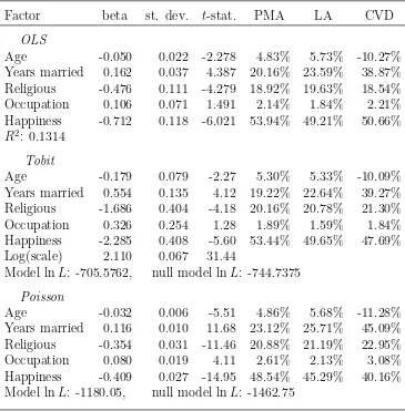
Econometric attribution is studied here in the context of Fair’s (1978) study of 601 responses of first-time married individuals to a 1969 sex survey conducted by Psychol-ogy Today. Fair studies the predictors of the frequency of marital infidelity. Green (2003) reanalyzes this publicly available data. Fair’s original model is first analyzed using OLS, tobit and Poisson regression. The determinants of marital happiness are then examined with OLS and ordered probit. In addition to model results, LAs, PMAs and covariance decompositions (CV Ds) are reported.4
3
A linear model without an intercept is a simple example.
4
CVD is a standard approach to variance decomposition in economics and finance. The CVD component of a factoriisβi1′NΣβ, whereβis the model coefficient vector, Σ is the factor covariance
matrix and 1N is a n×1 vector of ones. See Feldman (2005a) Sections 4.3, 4.4 and 5 for results
Factor beta st. dev. t-stat. PMA LA CVD
OLS
Age -0.050 0.022 -2.278 4.83% 5.73% -10.27%
Years married 0.162 0.037 4.387 20.16% 23.59% 38.87%
Religious -0.476 0.111 -4.279 18.92% 19.63% 18.54%
Occupation 0.106 0.071 1.491 2.14% 1.84% 2.21%
Happiness -0.712 0.118 -6.021 53.94% 49.21% 50.66%
R2: 0.1314
Tobit
Age -0.179 0.079 -2.27 5.30% 5.33% -10.09%
Years married 0.554 0.135 4.12 19.22% 22.64% 39.27%
Religious -1.686 0.404 -4.18 20.16% 20.78% 21.30%
Occupation 0.326 0.254 1.28 1.89% 1.59% 1.84%
Happiness -2.285 0.408 -5.60 53.44% 49.65% 47.69%
Log(scale) 2.110 0.067 31.44
Model lnL: -705.5762, null model lnL: -744.7375
Poisson
Age -0.032 0.006 -5.51 4.86% 5.68% -11.28%
Years married 0.116 0.010 11.68 23.12% 25.71% 45.09%
Religious -0.354 0.031 -11.46 20.88% 21.19% 22.95%
Occupation 0.080 0.019 4.11 2.61% 2.13% 3.08%
Happiness -0.409 0.027 -14.95 48.54% 45.29% 40.16%
[image:19.612.123.488.84.455.2]Model lnL: -1180.05, null model lnL: -1462.75
Table 2: Reanalysis of Fair (1978). Independent variable: frequency of infidelity.
The response variable studied by Fair is the self-reported frequency of infidelity. The explanatory factors include the respondent’s sex, age, education and occupation, the number of years married, whether the respondent has children and the respon-dent’s (self reported) level of religious belief and marital happiness.5
Fair excludes sex, education and having children as predictive factors based on their joint statistical insignificance. In attributions based on the complete model, all attribution methods assign these factors small attribution components, consistent with their low individual test statistics. The respective t-statistics are (0.18, 0.41, 0.21). The corresponding PMA components are (0.03%, 0.21% 0.05%). PMA and
t-statistics can together better motivate efficient multivariate hypothesis testing than
t-statistics alone. LA results, (0.15%, 3.12%, 0.29%), are not as clear for education.
5
Factor beta st. dev. t-stat. PMA LA CVD
OLS
Sex -0.070 0.103 -0.69 1.45% 0.75% 0.27%
Age -0.006 0.008 -0.78 4.33% 19.92% 11.25%
Years married -0.035 0.014 -2.52 58.54% 35.13% 48.50%
Children -0.207 0.120 -1.74 10.74% 19.83% 18.63%
Religious 0.085 0.038 2.22 7.17% 5.44% 2.43%
Education 0.074 0.022 3.41 16.08% 17.71% 19.73%
Occupation -0.025 0.030 -0.83 1.69% 1.21% -0.81%
R2 : 0.0894
Ordered probit
Sex -0.092 0.106 -0.86 2.09% 1.04% 0.92%
Age -0.005 0.008 -0.68 3.21% 19.72% 9.70%
Years married -0.037 0.014 -2.60 58.64% 36.18% 49.57%
Children -0.262 0.125 -2.09 15.60% 23.18% 23.82%
Religious 0.087 0.039 2.20 6.87% 5.16% 2.07%
Education 0.069 0.022 3.10 12.08% 13.70% 14.31%
Occupation -0.025 0.031 -0.81 1.51% 1.03% -0.40%
[image:20.612.118.494.81.388.2]Model lnL: -1180.05, null model lnL: -1462.75
Table 3: Data from Fair (1978). Independent variable: Self-rated marital happiness.
Table 2 presents results based on Fair’s original model. Factor coefficients are not directly comparable, Greene (2003) discusses the expected relationships. OLS and probitt-statistics are similar. Poisson factort-statistics are considerably higher. Age and happiness reduce infidelity, but years married increases it.
PMA, LA and statistical significance rankings are identical in this case. CVD consistently finds year married about twice as important as PMA or LA. CVD also finds years married more important than happiness in the Poisson regression. Model choice, in this case, affects coefficients and their precision, but has little effect on LA, PMA or the relative magnitudes oft-statistics. Note that LA and PMA give identical results when factors are uncorrelated. CVD results then also agree for OLS.
The negative CVD components for age in all models are problematic and causes the high CVD importance of years married. When age is removed from the OLS model of infidelity the CVD relative importance of years married falls to 25%, and that of happiness rises to 53%, similar to PMA and LA results.
increase in the LA component is just above 15%. Explained variance is proportional to the square of the beta in uncorrelated OLS, which would imply a 69% increase.
For the OLS and ordered probit models of marital happiness, all attribution meth-ods indicate years married is most important. The bootstrap probability that PMA years married is larger (more important) than PMA education is greater than 85%. In contrast,t-statistics seem to show education is most precisely estimated. In practice, this result is commonly interpreted as indicating that education is most important.
Age and years married are highly correlated (ρ=.78), which degrades statistical test values. Indeed, when age is excluded the years marriedt-statistic becomes largest (-4.44 for OLS). Age, however, may be a valid predictor for marital happiness. If so, its exclusion from the model could bias the model and attribute its explanatory power to the factors with which it is most correlated. Also, the LA for years married rises to 51% when age is excluded, indicating the relative sensitivity of LA to model definition. An F-test of the joint significance of sex and age in the OLS model is rejected (p=0.76). But removing age increases the magnitude of the years married beta by 22%. It would be a mistake to exclude age if the goal was to obtained unbiased coefficient estimates unless it could be maintained that age did not belong in the model in the first place. The age PMA of 4.33% signals this result.
4
General microeconomic models
4.1
Inert factors and utility attribution
Is random order consistency an acceptable axiom for utility attribution? Consider this question in the context of portfolio optimization. Uncorrelated assets, e.g., risk-free assets, are not inert factors: Their utility contribution is not independent of other assets. Further, an investment option of zero utility cannot be inert by definition.
The ability to define an inert factor must thus rely on a factor that is not a portfolio choice. Its utility must be independent of the portfolio. These conditions are satisfied if utility is additively separable in the investment and the inert factor.
There is no reason why two completely independent choice problems could not, in principle, be composed into a single optimization problem. This simple fact appears to allow the definition of an inert factor in almost any choice problem. Random order consistency becomes applicable once it is established the existing attribution problem could be composed with a suitable independent problem as a larger attribution.
Risk and return Correlation
Asset Mean Std. Sharpe LC SC Intl Gvt Corp Bills
Large Cap 0.0106 0.041 0.258 1.000 0.729 0.619 0.116 0.217 0.069
Small Cap 0.0110 0.053 0.209 0.729 1.000 0.529 -0.015 0.110 -0.053
Int’l 0.0062 0.048 0.128 0.619 0.529 1.000 0.009 0.082 -0.068
LT Gvt. 0.0082 0.026 0.320 0.116 -0.015 0.009 1.000 0.948 0.079
LT Corp. 0.0079 0.021 0.384 0.217 0.110 0.082 0.948 1.000 0.069
[image:22.612.90.535.84.213.2]T-Bills 0.0037 0.002 — 0.069 -0.053 -0.068 0.079 0.069 1.000
Table 4: Asset performance data, monthly 1988-2004.
4.2
Portfolio attribution
Let N be a set of n assets with expected return vector µ and covariance matrix Σ. Using quadratic utility and formula (1), v(S) for any set of assets S is
vmvo(S) = U(S)−U(∅) = max(0, max
ωS∈∆S
ωS′µS−λωS′ΣSωS), (16)
where λ is the index of quadratic risk aversion, µS, ωS and ΣS are restricted to the
members of S, ωS is the portfolio allocation and ∆S is thes−1 dimensional simplex
of nonnegative portfolio weights that sum to unity. Here U(∅) = 0. The restriction
v(S)≥ 0 allows not investing if v(S) < v(∅), as is possible when restricted to some asset combinations. If exponential utility were used, then U(S) < 0 for all S ⊆ N
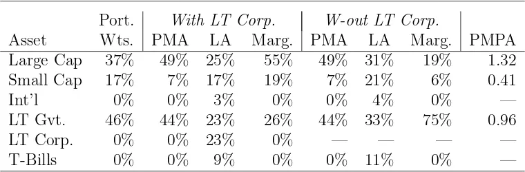
and the definition v(S) = U(S)−U(∅) is necessary, as in Section 3.2 for likelihoods. Table 4 reports the assets used in this example, along with their monthly mean total returns, standard deviations, Sharpe ratios and correlations for the period 1988 to 2004.6,7 Table 5 presents the optimal portfolios for an individual with quadratic
risk aversion levelλ = 2, along with two sets of attributions. One is for all investment options. The other excludes corporate bonds. For each set, PMA and LA results and (discrete) marginal utility contributions are reported. All attributions are normalized to 100%. The final column of Table 5 presents the proportional marginal performance attribution (PMPA) of assets with positive portfolio allocations. The PMPA of an asset is the ratio of its PMA to its portfolio weight.
6
Monthly data from Ibbotson Associates covers the period January 1, 1988 to December 31, 2004. Large cap is the S&P 500, small cap is the Russell 2000, international is the MSCI Europe, Asia and Far East Index, long-term government is the Ibbotson U.S. Long-Term Government Bond Index, long-term corporate is the Ibbotson U.S. Long-Term Corporate Bond Index and t-bills is the Ibbotson U.S. 30 Day T-Bill.
7
Port. With LT Corp. W-out LT Corp.
Asset Wts. PMA LA Marg. PMA LA Marg. PMPA
Large Cap 37% 49% 25% 55% 49% 31% 19% 1.32
Small Cap 17% 7% 17% 19% 7% 21% 6% 0.41
Int’l 0% 0% 3% 0% 0% 4% 0% —
LT Gvt. 46% 44% 23% 26% 44% 33% 75% 0.96
LT Corp. 0% 0% 23% 0% — — — —
[image:23.612.116.496.84.209.2]T-Bills 0% 0% 9% 0% 0% 11% 0% —
Table 5: Asset allocation and performance attribution when λ= 2.
The optimal portfolio monthly return and standard deviation are 0.0096 and 0.026 and its Sharpe ratio is 0.364. It is about 54% equity and 46% fixed income. The PMA is in similar proportion (56%/44%). Only assets with positive portfolio weight receive a PMA share, while every asset class receives some LA share. LA gives government and corporate bonds almost equal importance even though corporate bonds receive no portfolio weight. Marginal contributions are heavily weighted to equity because of the substitutability of government and corporate bonds.8
PMPA provides a measure of an asset’s per dollar contribution to portfolio per-formance. The PMPA ranking is differs from the Sharpe ratio ranking. Government bonds have the highest Sharpe ratio of all allocated assets, followed by large cap equity. But Large cap equities contribute most to portfolio performance per unit of investment. The PMPA of large cap equity is more than three times the PMPA of small cap equity even though its Sharpe ratio is only 23% higher. The Sharpe ratio measures stand-alone performance, whereas PMPA evaluates performance relative to a specific portfolio. (Note, corporate bonds have the highest Sharpe ratio but receive no asset allocation.) Further, attribution is relative to a specific risk profile.
In the second set of attributions of Table 5, corporate bonds are not an option. The PMA does not change. The LA equity share rises to 52%, but now government bonds are seen as more important than large cap equity. The relative marginal contribution of government bonds is now very high without substitution from corporate bonds, and equity marginal contribution is weak because of equity mutual correlation.
If t-bills and international equity are also removed from the choice set, the LA becomes (37%,25%,28%) and equity receives 62% total attribution. PMA results are unchanged. When large cap and small cap shares are aggregated, the PMA is (52%, 48%) and the LA is (53%, 47%). In all cases, PMA implies that a little over
8
half of portfolio performance is attributable to equity and almost half to bonds. LA implications depend strongly on details of the attribution analysis.
Unutilized assets are irrelevant for PMA because of exclusion. In this example, and generally, PMA is not very sensitive to aggregation; but it is possible to construct contrary examples. Linear attribution is sensitive to both unutilized factors and factor aggregation (as in example 5.1, below). The differences between LA and PMA may be a useful measure of the substitutability of factors. PMA offers a consistent method of attributing joint effects in the creation of investment value, and thereby providing insight into its sources.
5
Joint cost attribution
Cost allocation has traditionally been considered a bargaining problem by game the-orists. In cost attribution, the utility function of formula (1) is an aggregate cost (disutility) function. The arguments of the cost function are typically aggregate de-mands for products or services over cost centers. The applicability of random order consistency to cost attribution raises the same types of issues as considered for utility attribution in Section 4.1. The potential existence of an inert cost center is no differ-ent the potdiffer-ential existence of an inert factor in a utility or econometric attribution.
5.1
Linear or proportional marginal cost attribution?
Neither inclusion nor exclusion appear obviously appropriate for cost attribution. While exclusion might seem appropriate for the attribution of profits, many might find it problematic that somebody is getting something for nothing. Exclusion in cost allocation requires that a party that imposes no final marginal cost should have no attributed cost if all other parties impose final marginal costs.
Inclusion may appear an innocuous axiom in this context, however linear cost allocation methods have not been widely adopted and were not well-received by ac-counting researchers. Moriarity (1975), Banker (1981) and Gangolly (1981) explicitly support or propose proportional alternatives. Banker writes that linear attribution is “not consistent with our axioms, and hence with traditional cost allocation methods.” (1981:127). Thomas (1977) provides examples that demonstrate the vulnerability of linear attribution to strategic definition of cost centers.9
Example 5.1 The potential for strategic manipulation in cost attribution is illus-trated in a simple sunk cost attribution problem. Assume n cost centers, sunk cost
C and fixed marginal cost c. Cost center i has usage xi. The cost of service to any
9
coalition of centers S is v(S) =C+cP
i∈Sxi. The marginal cost of any coalition of
centersS 6=N, is represented in the dual game by w(S) = cP
i∈Sxi. Thus, the game
w(S) is additive for all S(N: w(S) =P
i∈Sw(¯i).
Lemma 2.2 implies P M Ai = ϕ(w)i = C/xi because w can seen as a rescaling of
w∗(N) in a w∗ where w∗(N) = cP
i∈Nxi. Similarly, LAi = cxi +C/n. When C is
very small, LA and PMA are approximately the same since then v(N)≈ cP
i∈N xi.
However, allocations diverge as C increases. When cP
i∈Nxi ≪ C, LA for all
centers approaches C/n, regardless of the disparities in usage between cost centers, providing incentive for group managers to aggregate reporting units.
Corollary 5.1 The proportional marginal share of costs attributed to any cost center is invariant with the magnitude of the fixed costs when fixed costs are scale invariant.
6
Discussion and conclusion
This paper introduces a new expectation-based random order approach to cooperative value. Linear and proportional value are characterized in a common setting without assuming linearity or proportionality. Random order consistency, the key element of this approach, assumes only that we can see the “expectational mechanics” of the random order process, and that these mechanics do not change if invisible inert players or factors are added. These mechanics have specific interpretation regarding the relative importance of factors in the theory of attribution developed here.
Random order consistency is key to both theoretical and applied results. Contrast this with the limited power of reduced game consistency discussed in Remark 1.1. Random order consistency is strongly and uniquely associated with cooperative value.
Consider the scope of this theory if based on reduced game consistency. The use of reduced game consistency must imply some correspondence between the reduced game and the original attribution. But few, if any, properties of a game or cost function are preserved by reduction. The reliance on the dual game is also problematic. Consider an attribution problem with a vector of demandsxand cost functionc(y) = yα,α 6= 1, so w(S) =c(xN)−c(xN\S) = [Pi∈Nxi]α−[Pi∈Sxi]α. Let w∗ be the game resulting
from the reduction of player k, so that N∗ =N \k¯ and w∗(S) =w(S∪k¯)−φ k(w),
where φi(w) is Shi(w) or ϕi(w). In general, there will be no vector of demands x∗
such that w∗(S) = c(x∗
N∗)−c(x∗N∗\S) for all S. Nor, in general, will there be a cost
function c∗ such that w∗(S) =c∗(x∗
N∗)−c∗(x∗N∗\S) for all S.10
Random order consistency places minimal demands on the structure of an attri-bution problem. Section 4.1 proposes it appropriate for any attriattri-bution problem that can be composed with an independent attribution.
10
The specific applications studied here demonstrate practical potential applica-tions. PMA appears to provide theoretically sound measures of the econometric relative importance of model independent variables. These measures also appear to allow comparison of relative importance across models and to be useful diagnostics for model construction and evaluation. Feldman (2005a and 2006) applies a similar approach with financial factor models to provide variance decomposition of an asset manager’s return stream to identify the relative importance of factor drivers.
The portfolio attribution example shows the considerable knowledge of data and preferences necessary for utility attribution, but, also, the potential benefit. Portfolio PMA and PMPA are new investment analysis tools and examples of practical feasible applications. They are distinctive in that they evaluate an asset’s total, as opposed to marginal, performance both relative to a portfolio and an investor’s risk preferences.
In this theory of attribution, linear and proportional value emerge as parallel expressions of an underlying value principle. This relative importance approach to cooperative value is developed specifically for the single-utility function attribution environment, but applies directly to TU bargaining as well. Feldman (2002) develops similar results for the more general nontransferable utility (NTU) games using ratio potentials. In this “dual” approach to value either the linear or proportional “mode” might be more appropriate for a particular application.
Game theoretic interest in proportional solutions, including the proportional value, has been hampered by the belief that they are translation dependent (see, e.g., Hart and Mas-Colell (1988: 595n)). Real allocations seem to change with affine translation of a player’s utility function. This outcome should arouse scrutiny as it implies the incoherence of a basic distributive principle recognized at least since Aristotle.11
The apparent translation dependence of proportional solutions results from a miss-ing element in the standard NTU cooperative game. Thebasis point, a vector of util-ities, one for each player, allows determination of the marginal utility to any player of any bargaining outcome. Feldman (2005b) demonstrates the existence of the basis point and shows that proportional solutions are translation invariant when a player’s basis utility and utility function are subjected to the same affine transformation.12
This theory of attribution is based on a single decision maker and, hence, would be unaffected even if proportional bargaining solutions were translation dependent. Examples presented here clearly demonstrate the relevance of the basis point in at-tribution problems. Section 3.2 shows that econometric atat-tributions are not uniquely defined unless the null model objective function value can be defined and used as the basis point. (Interestingly, PMA shares are invariant to the choice of the basis point.) Similarly, Section 4.2 shows that utility attribution must specifically define null model utility for utility functions where null model utility is not zero.
11
Young (1994: 64) writes “[p]roportionality is deeply rooted in law and custom as a norm of distributed justice.” Moulin (1999) starts by quoting Aristotle: “Equals should be treated equally, and unequals, unequally in proportion to relevant similarities and differences.”
12
Finally, researching the accounting literature, I was often surprised by the inten-sity of the arguments against linear cost allocation, and sometimes by the palpable frustration. Thomas (1977: 43), in his study of cost allocation and transfer pricing, chooses the following epigraph (from Lousia M. Alcott’sJack and Jill) for his chapter on cost allocation using the Shapley value: “. . . Molly retired to wet her pillow with a few remorseful tears, and to fall asleep, wondering if real missionaries ever killed their pupils in the process of conversion.” Neutrality between linear and proportional methods is theoretically sound and evolutionarily wise.
7
Proofs
7.1
Appendix A: Proof of Lemma 1.1
Proof: I. First consider multiplicative likelihoods. Endogenous random order con-sistency requires that functions of the worths of factor sets including an inert fac-tor facfac-tor out of the sum of likelihoods generated by a suborder. The terms in
P
r⊃ro
Q
i∈Nli(w(Sir)) do not factor directly. An alternate approach is required.
Consider a single inert factor z ∈ N. Select any r0 in R(N \ z¯). By
insert-ing z at all possible positions in r0, all orders in N that include r0 are generated.
Define ri
0 ∈ R(N) as the order resulting when z is inserted at the ith position:
ri
0 = (r01, . . . , r0i−1, z, r0i, . . . , r0n−1). Then let R
∗ ={ri
0}ni=1 = (r10, r02, . . . , r0n).
Define ¯S as all nonempty factor sets included in r0, so that ¯S = {S :S ⊂ r0}= {Sr0
i }n−i=11. Let ¯Sz contain the singleton ¯z and the union of each factor set in ¯S with
z: ¯Sz ={S :S =T ∪z, T ∈S¯ orT =∅}. Index the members of ¯S and ¯Sz by their
cardinality: ¯S3 has cardinality three. Define S∗ = ¯S∪S¯z.
Set of setsS∗ helps to form a common denominator for multiplicative likelihoods.
For any ri
0 ∈R∗, let R∗i be the factor sets that are included in ri0: R∗i ={S|S ∈r0i}.
R∗
i ⊂ S∗. Define Ti∗ as the sets in S∗ not included in ri0: Ti∗ = S∗ \ R∗i. Let
K =Q
S∈S∗li(S)−1, wherei is the cardinality of S. Then, for alli∈N,
L(ri0) =
Y
S∈ri
0
li(S) =
1
K
Y
S∈T∗
i
li(S)−1 ≡
1
KLˆ(r
i
0), (A1)
where ˆL is a partial likelihood with ˆLi =l−i 1. For every j < n there are two sets in
S∗ with j factors. Only one of these factor sets is in any T∗
i . These are Sjro = ¯Sj
and ¯Sz
j = Sj−ro1∪z. If one is in R∗i then it is not in Ti∗, and vice-versa. For j < i,
¯
Sz
j ∈ Ti∗ because ¯Sj ∈ R∗, and for j ≥ i, ¯Sj ∈ Ti∗ because ¯Sjz ∈ R∗. Thus, Ti∗ =
{S¯z}i−1
Let T∗i
j be the factor set in Tj∗ of cardinality i. Then
ˆ
L(r10) + ˆL(r02) =
n−1
Y
i=1
li(T1∗i)−1+
n−1
Y
i=1
li(T2∗i)−1
= ³l1( ¯S1z)−1+l1( ¯S1)−1
´n−Y1
i=2
li( ¯Si)−1.
When w( ¯Sz
1) = w(¯z) > 0 factorization requires l1(S) = l2(S) = w(S)−1. Then
l(S)−1 = w(S) and, since z is inert, w( ¯Sz
2) = w(¯z) + w( ¯S1). Note that any l with
l(0) =∞ trivially allows factorization if w(¯z) = 0. (Thus the requirement that inert factors have positive individual worth.) If and only if l1(S) = l2(S) = w(S)−1 can
these terms be combined and absorbed into the product
ˆ
L(r10) + ˆL(r02) =w( ¯S2z)
n−1
Y
i=2
li( ¯Si)−1.
Induction is used to sum likelihoods. Assume that li(S) = w(S)−1 for all i < j
and that the following pattern holds for sums of the first j −1 orders in R∗:
j−1
X
i=1
ˆ
L(r0i) =
j−1
Y
i=2
w( ¯Siz)
n−1
Y
i=j−1
li( ¯Si)−1.
Under the above assumptions, ˆL(rj0) may be written
ˆ
L(rj0) =
j−1
Y
i=1
w( ¯Siz)
n−1
Y
i=j
li( ¯Si)−1.
Adding and factoring the last two expressions gives the first formula below. The second follows if and only if lj(S) =w(S)−1. The induction is a “zipper.”
j
X
i=1
ˆ
L(r0i) = ³w( ¯S1z) +w( ¯Sj−1)
´j−Y1
i=2
w( ¯Siz)
n−1
Y
i=j
li( ¯Si)−1
=
j
Y
i=2
w( ¯Siz)
n−1
Y
i=j
li( ¯Si)−1 (A2)
Evaluating (A2) atj =n and recalling (A1) and that ¯S ={S :S ∈ro} gives
1 K n X i=1 ˆ
L(r0i) = 1
K
n−1
Y
i=2
w( ¯Siz) = w(¯z)−1 Y
S∈r0