An econometric approach to robust identification for models of inverse dynamic problem

Munich Personal RePEc Archive

An econometric approach to robust

identification for models of inverse

dynamic problem

Filchenko, Dmytro / D.

Sumy State University

2007

Online at

https://mpra.ub.uni-muenchen.de/30761/

УДК 330.43

D.V. Filchenko

A Game-Theoretical Specification of Static Optimization Problems

for the First-Order Lag Models of Macroeconomic Dynamics

In most cases macroeconomic models describe the overall economy within a dynamic framework. That means that along with static elements such models contain at least one dynamic element within either discrete or continuous time span. Basically, for numerical computations any differential equation is always transformed into a difference one. Thus further we will consider models in the form of finite-difference equations.

The problem of dynamic optimization is widely explored and has a lot of applications in macroeconomic modeling [1]. It is also probable to specify static optimization problems using a dynamic framework. Particularly, such problems appear as different facets of efficient resource allocation [2, 3].

Due to [4], let us assume that dynamics of n-industrial open macroeconomic system can be described by a system of difference equations. It has the following matrix form (for N discrete points of time):

)) ( ( )) ( ( ) ( ) 1

(t x t µ x t λ u t

x + − = + , {t = 0, 1, …, N-1} (1)

where x = (x1, x2, …, xn, xn+1)tr is a vector of phase coordinates in which the first n variables are fixed capital accumulations per industry, and xn+1 is a foreign debt; u(t) = (u1, u2, …, ul)tr is a vector of foreign and domestic investment flows. µ(⋅) and λ(⋅)are vector-valued functions:

n i i} 1

{µ = is a set of amortization functions; µn+1 is a debt services function [5]; 1 1

}

{λi ni=+ states

for functions which describe how gross investments impact left-hand side of (1), i.e. either net investments for {i = 1, 2, …, n} or foreign debt gross accumulation for i = n+1. For the sake of simplicity, in most applications [6, 7] vectors µ(⋅) and λ(⋅⋅) may be considered as linear functions, so that (1) takes a form of

) ( ) ( ) ( ) 1

(t x t Mxt Λu t

x + − = + , (2)

where M is a (n+1)×(n+1) diagonal matrix of constant coefficients (with negative signs, except the last) and Λ is a (n+1)×l non-diagonal matrix of weight coefficients.

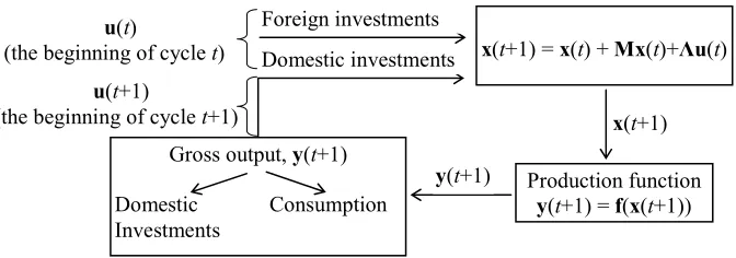
The dynamic model (2) can be viewed as a combination of the following elements [3]. Vector-valued functions µ(x(t))=Mx(t) and λ(u(t))=Λu(t) are zero-order static elements called multiplicators. A Sub-model x(t+1)−x(t)≈Λu(t) is a zero-order dynamic element called an accelerator. It describes the proportional relationship between gross investments (outputs) and the rate of inputs. The model (2) itself can be considered as another structural element known as a first-order time lag (inertia) element. Its inputs are corresponded gross growth values and outputs are corresponded accumulations, and it represents the ‘working-off’ of the inputs.

u(t)

(the beginning of cycle t)

u(t+1)

(the beginning of cycle t+1)

x(t+1) = x(t) + Mx(t)+Λu(t)

Production function

y(t+1) = f(x(t+1)) Gross output,y(t+1)

Domestic Consumption Investments

Domestic investments Foreign investments

x(t+1)

y(t+1)

Figure 1 Structure of a modified Solow’s first-order lag model

Now we start with the mechanism of transforming the dynamic model (2) into N static optimization models.

Suppose that for each of n industries there is available statistical information about fixed capital accumulations {xi(t)}ni=1 and coefficients of amortization

n i i

m} 1

{ ₌ , foreign debt accumulation xn+1 and coefficient of debt services mn+1. The identification of matrix Λ will be considered later. Hence u(t) {} 01

− = N t

t are the only unknown parameters. Consequently, (2) is a system of n + 1 linear algebraic equations with l variables.

Further we will consider the situation when l > n+1, which corresponds to economic reality most of all. In this case, when the system is overdetermined, there appears some arbitrariness in the model. Using l-n-1 numbers of freedom, one can provide an effective structure of unknown vector u(t).

Coordinates {u_j}l_j=1 can be always renumbered so as the first l-n-1 variables are free, while the others n+1 are basic. Then basic variables are expressed in terms of free variables:

u2(t) = (Λ2(t))-1 (x(t+1) – x(t) – Mx(t)–Λ1(t)u1(t)), (3) where u1(t)=(u₁(t),u₂(t),...,u_l−n−1)tr, u2(t)=(u_l−n−1(t),u_l−n(t),...,u_l)tr, Λ1 and Λ2 are

(n+1)×(l–n–1) and (n+1)×(n+1) matrices of weight coefficients.

Now let’s turn to matrix Λ(t) identification. Consider an open macroeconomic system, every i-th {i}n_i=1 industry of which produces both final consumption and investment goods. The sum of all outputs form a total output, or GDP Y(t). All goods are both exported and imported. Let vector u(t) contains the following coordinates: u1(t), u2(t), …, un(t), foreign investment flows per industry; un+1(t), un+2(t), …, u2n(t), domestic investment flows per industry; and u2n+1, the sum of net exports and domestic investments abroad. So in this case l, the number of the unknowns, is 2n+1, and (3) has n degrees of freedom. Then the matrix Λ(t) may be identified as follows:

Λ(t) = (Λ1(t), Λ2(t)),

n n t 1 _ _ ) ( _⎟⎟ ⎠ ⎞ ⎜ ⎜ ⎝ ⎛ = i I Λ1 , ) 1 ( ) 1 ( ) ( + × + = n n t I Λ2 , (4)

where I is an identity matrix, i is a vector of unities.

) (

max 1

u

u

1 F

subject to h(u1)≤c,

where F(·) is an objective function, h(·) is a constraint vector-valued function, c is a vector of constraint coefficients.

Suppose that the process of investment development is the process of two aggregate players’ interaction: a recipient (national economy) and a foreign investor. Let a recipient have n pure strategies (n absolute priorities per industry), while an investor can operate with n+1 pure strategies (being specialized either in the i-th industry {i}n_i=1 or in diversification policy, i.e. to invest into each of n industries). If a recipient’s strategy does not coincide with that of an investor, then both will gain nothing. Otherwise, a recipient’s payoff is investments obtained into the i-th industry at time t, and an investor’s payoff is the sum of profits he can receive during some future periods. These two payoffs are separated in time. Therefore, using a net presence value, an investor’s payoff should be discounted to initial time t.

Specified game is a static game with simultaneous moves. It has two solution concepts: Nash equilibrium (in pure strategies) and mixed Nash equilibrium (in mixed strategies). Any pure strategy however reflects in a trivial situation, when only the one industry is invested. Thus, further mixed strategy is considered.

Let p = (p1, p2, …, pn) be a vector of probabilities ( 1 1

=

∑

n

i i

p ). Each {pi}in=1 states for

probability of choosing the i-th strategy by a recipient. Suppose also that an investor chooses strategy of diversification. Consequently, a recepient’s expected payoff (i.e. mathematical expectation of payoff) is pu1. Therefore, it is natural to specify the objective function F(·) as follows:

1

u

1 _pu

u

1

=

) (

max F . (5)

As to h(·) and c specification, for the sake of simplicity we will elaborate two possible constraints. The first one naturally follows from the fact that total foreign investments can not exceed some critical value Icr:

cr I

≤

1

iu . (6)

In order to obtain the second constraint, let k(t) be a coefficient that shows what part of domestic consumer goods should remain for domestic consumption; ki(t) be a part of domestic investments un+i(t) in the i-th industry that should remain for domestic development. Using (3), (4), we arrive at the following constraint at time t [12]:

( ) (

)

(

)

(

)

As a result, choosing mixed strategy, a recipient encounters linear programming (LP) problem (5)-(7) at every point of time. The opportunity set of the specified LP problem intercepts a n-dimensional coordinate system at some points which correspond to the case of pure strategies. Let us designate theses points as I1, I2, …, In.. Then if the recipient is rational, we can derive a condition of choosing mixed strategy by him:

Consider the problem of optimal investment allocation using two-industrial (n = 2) Danish economy in 1966-1997 as an example. Let the first industry consist of manufacturing and agricultural branches and the second one of services branches. The statistic analysis [10, 11] reveals that parameters k(t), k1(t), k2(t) may be considered as constants equaled to 0.93, 0.98, and 0.80 correspondently. Take note of essential difference between the parts of investment goods from the first industry aimed to be exported (2%) and the same for the second industry (20%). The latter generally corresponds to results that will be obtained further.

For the degree of freedom l-n-1 = 2 conditions (8) can easily take form

(

)

⎠ ⎞ ⎜

⎜ ⎝ ⎛

< < <

= <

2 1

1 2 1

1 2

/ /

1 &

I I p p I

I I

I _cr ,

where / 1

I is the solution of (7) subject to u2 = 0.

As a result, the priorities p1 and p2 of investment development should be chosen as 0.44 and 0.56 correspondently. Then using the LP model (5)-(7), optimal investment allocation can be computed at each of N points of time t (for details see [12]). Time-series trends of real and optimal (designated with an asterisk) investments are derived employing OLS estimation [13]:

* 1

ˆ

u (t) = 1.70t4 – 97.22t3 + 1639.96t2 – 6208.48t + 8758.67, R2 = 0.95;

1 ˆ

u (t) = 1.41t4 – 73.84t3 + 1086.26t2 – 2013.09t + 6037.72, R2 = 0.92; *

2 ˆ

u (t) = 1.44t4 – 82.64t3 + 1392.64t2 – 5288.82t + 7426.48, R2 = 0.95;

2 ˆ

u (t) = 0.69t4 – 37.06t3 + 540.04t2 – 319.32t + 1861.06, R2 = 0.92.

The coefficients of determination R2 for optimal trends appear to be higher than those for real trends. Particularly, this can be a result of better stability of economic system under the optimal investment allocation.

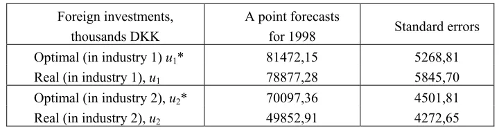
Extrapolation [14] of defined trends leads to the table below. The optimal plan of foreign investment allocation for 1998 implies more expansive investment policy, especially for services. While the second industry appears to be more developed and have the higher priority (p2 > p1), foreign investments are more demanded by the first industry. This results in a substantial misbalance of investment exports and higher fulfillment of investment market with domestic investments.

Table – Optimal and real allocations of investments. Forecast values

Foreign investments, thousands DKK

A point forecasts

for 1998 Standard errors

Optimal (in industry 1) u1* 81472,15 5268,81

Real (in industry 1), u1 78877,28 5845,70

Optimal (in industry 2), u2* 70097,36 4501,81

Real (in industry 2), u2 49852,91 4272,65

optimization model. Specifically, using game theory tools, we shifted from the dynamic model of investment development to the static models of optimal investment allocation between two industries. All modes were approbated using two-industrial open macroeconomic model of Danish economy. Retrospective analysis revealed correspondence with reality and possibility for the future corrections of investment policy, while prospective analysis gave implicit recommendation about optimal strategies in forecast periods. Nevertheless, it should be noted that no optimal policy obtained analytically can be considered as the only one. Any analytical solution is a complimentary descriptive characteristic of the system that describes an ideal optimality of instrumental variables.

1. Ljungqvist L., Sargent T. Recursive macroeconomic theory. Second edition. – Massachusetts

Institute of Technology, 2000. – 988 pp.

2. Intriligator M.D. Mathematical optimization and economic theory. – Philadelhia, PA: Society for

Industrial and Applied Mathematics, 2002. – 508 pp.

3. КолемаевВ.А. Экономико-математическое моделирование. Моделирование макро

-экономическихпроцессовисистем. – М.: Юнити, 2005. – 295 с.

4. НазаренкоО.М. Динамічне моделювання інвестиційного розвитку та оптимальної

макроекономічної інвестиційної політики // Механізм регулювання економіки. – Суми:

Університетськакнига, 2006. – №4. – С. 187-195.

5. Romer D. Advanced Macroeconomics. – Blacklick, OH: McGraw Hill, 1996. – 540 pp.

6. ДикусарВ.В., СинягинС.Ю. Качественные и численные методы в задаче оптималь-ного

управлениявнешнимдолгом: Сообщ. поприкл. матем. // ВЦРАН. – М., 2000.

7. Obstfeld M., Rogoff K. Foundations of International Macroeconomics. – The MIT Press, 1996. – 790

pp.

8. Turnovsky S. J. Methods of Macroeconomic Dynamics (2nd. ed.). Cambridge, Mass.: The MIT

Press, 2000. – 365 pp.

9. ФільченкоД.В., НазаренкоЛ.Д., НазаренкоО.М. Особливості побудови та верифікації

ймовірнісно-статистичних моделей макроекономічної динаміки // Вісник Криворізького

економічногоінституту. – КривийРіг, КЕІКНЕУ, №1, 2007. 10.Denmark Statistics: http://www.dst.dk.

11.OECD, Statistic database: http://www.oecd.org.

12.НазаренкоО.М., ФільченкоД.В. Оптимальнийрозподіл інвестиційнихпотоків удинамічній

моделі макроекономічної системи // Фізико-математичне моделювання та інформаційні

технології. – Львів: Центр математичного моделювання інституту прикладних проблем

механікиіматематики, вип.7, 2007. – С. 5-16.

13.Greene W.H. Econometric analysis. Fifth Edition. – New Jersey: Prentice Hall Upper Saddle River,

2003.

14.НазаренкоО. М. Основи економетрики: Підручник. – Київ: „Центрнавчальної літератури”, 2004.

Д.В. Фильченко

Теоретико-игроваяспецификациязадачстатическойоптимизации

длямоделеймакроэкономическойдинамикислагомпервогопорядка

Изучена проблема перехода от моделей макроэкономической динамики в форме лагового элементапервого порядка к конечному числу моделей статической оптимизации. В качестве

динамическоймоделирассмотренамодельинвестиционногоразвития (типаСолоу), авкачестве

статической – модельоптимальногораспределенияиностранныхинвестицийвдвухотраслевой

открытоймакроэкономическойсистеме. Главныйинструментспецификациииидентификации

статическихоптимизационныхмоделей – аппаратстатическойтеорииигриматематического

Д.В. Фільченко

Теоретико-ігроваспецифікаціязадачстатичноїоптимізації

длямоделеймакроекономічноїдинамікизлагомпершогопорядку

В статтірозглядаєтьсяпроблема специфікаціїстатичноїоптимізаційної задачіврамках моделімакроекономічноїдинаміки. Базовоюдлядослідженнясталалінійнадискретнамодель (1)

інвестиційного розвитку відкритої n-галузевої макроекономічної системи. Головне завдання

роботи – теоретичне обґрунтування та практична апробація алгоритму трансформації в

кожний дискретний момент часу моделі (1), яка лише описує еволюцію макроекономічної

системи, вмодельстатичноїоптимізації. Вякостіостанньоїбулаобранамодельоптимального

розподілуіноземнихінвестиційміжгалузямиекономіки.

Ідеяпереходувіддинамікидостатикиполягаєвнаступному. Якщочислозміннихуправлінь (інвестиційних потоків) в системі різницевих рівнянь (1) більше, ніж число самих рівнянь, то

системавиявляєтьсяперевизначеною, асередчислазміннихможнавиділитибазиснітавільні.

Оскількиінструментальнізміні – іноземні інвестиційні потоки, тов роботі самевони обрані

вільними. Базисні змінні в будь-який момент часу за допомогою рівнянь системи (1) можуть

бутивираженічерезвільні.

Отже, залишається специфікувати оптимізаційний критерій та систему обмежень на

інструментальнізмінні. Процес інвестиційного розвитку макроекономічноїсистемив статті

розглянутий як процес взаємодії двох агрегованих учасників: реципієнта, або одержувача

інвестицій (національноїекономіки) таіноземногоінвестора. Булоприпущено, щореципієнтмає n чистихстратегій – віддаватиабсолютнийпріоритет i-йгалузі (i = 1, 2, …, n), аінвестор, в

своючергу, можеобиратиміж (n+1)-ючистимистратегіями – спеціалізуватисяна i-йгалузі

абождиверсифікуватиінвестиції, залучаючиїхвкожнугалузьекономіки.

Якщостратегіїреципієнтатаінвесторанеспівпадаютьдляжодноїзгалузей, виграшіобох

природнобудутьдорівнюватинулю. Якщожобраністратегіївідображаютьспільнийінтерес

гравців, то виграшреципієнтабудедорівнювати залученим інвестиціямв i-угалузь вмомент

часу t, авиграшінвестора – суміприбутків, яківінможеотримативідінвестуванняпротягом

кількохнаступнихперіодів (додеякогокінцевогомоментучасу). Цідвавиграшірозділенівчасі,

томулогічновиграшінвесторадисконтуватидомоменту t, використовуючивеличинучистого

теперішньогозначення. Проте, будь-якийрозв‘язокцієїгривчистихстратегіяхєтривіальним:

інвестуєтьсялишеоднагалузь. Томузапропонованозробитиперехіддозмішанихстратегій.

Припущено, щореципієнтобираєкожнусвоюстратегіюздеякоюймовірністю, аінвестор

диверсифікуєінвестиції. Тодіцільовафункція (5) відображаєочікуванийвиграш (математичне

сподіваннявиграшу) реципієнта. Длянаочностітакожзапропонованодваобмеження (6) і (7) на

змінні. що відповідають іноземним інвестиціям. Разом із умовою невід‘ємності

інструментальнихзміннихмодель(5)-(7) складаєзадачулінійногопрограмування.

Длятого, щобпозбутисядовільностіувиборіймовірностейвиборустратегійінвестування

галузей та величини граничного рівня іноземних інвестицій (яка з‘явилася в обмеженнях),

отримані умови (8) вибору реципієнтом змішаної стратегії. Якщо умови (8) виконані, то

оптимальнийрозв‘язокспецифікованоїзадачілінійногопрограмуваннябудевідповідатизмішаній

стратегіїреципієнта.

Апробація запропонованих моделейі підходів була здійсненана прикладіекономіки Данії у період 1966-1997 рр. Весь реальний сектор був умовно розділений на дві галузі: промислово-

сільськогосподарську і галузь послуг. Для кожного року були отримані оптимальні значення

іноземнихінвестицій для кожних з галузей, а також їх пріоритети розв‘язку. За допомогою

методу найменших квадратів отримані часові тренди реальних та оптимальних іноземних інвестиційдлязаданогоперіоду. Аналізвбазовийперіодєретроспективнимідозволяєвиявляти

причини відхилень реальних трендів від оптимальних та коригувати інвестиційну політику в майбутньому. У статті також пропонується можливий підхід до задачі планування (прогнозування) оптимальної інвестиційної політики (так званий, проспективний аналіз) за

допомогоюекстраполяціївиявленихтенденційметодомбезумовногопрогнозування.