Path Planning of Mobile Robot by using Modified
Optimized Potential Field Method
Alaa A. Ahmed
Department of Electrical Engineering, University ofBasrah, Basrah, Iraq
Turki Y. Abdalla
Department of Computer Engineering University ofBasrah, Basrah, Iraq
Ali A. Abed
(IEEE Member) Department of Computer Engineering, University ofBasrah, Basrah, Iraq
ABSTRACT
This paper deals with the navigation of a mobile robot in an unknown environment by using artificial potential field (APF) method. The aim is to develop a method for path planning of mobile robot from start point to the goal point while avoiding obstacles on robot’s path. Artificial potential field method will be modified and optimized by using particle swarm optimization (PSO) algorithm to solve the drawbacks such as local minima and improve the quality of the trajectory of mobile robot.
Keywords
Path Planning, Artificial Potential Fields, PID Controller, Particle swarm optimization
1.
INTRODUCTION
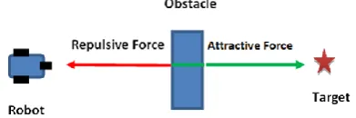
The goal of the path planning method is to determine a sequence of configurations for the robot to move around obstacles and avoid collisions while reaching a desired goal [1]. The artificial potential field (APF) method is widely used for planning the path of mobile robot. In the artificial potential field method, a mobile robot is considered to be subjected to an artificial potential force. The potential force has two forces: first one is attractive force and second one is repulsive force. In the artificial potential field method, we can imagine that all obstacles can generate repulsive force to the robot that is inversely proportional to the distance from the robot to obstacles and is pointing away from obstacles, while the destination or goal has attractive force that attracts robot to the goal. The combination of these two forces will generate a total force with magnitude and direction, the mobile robot should follow that direction to avoid obstacles and reach to the target in a safe path [2]. Actually the artificial potential field method uses a scalar function called the potential function [3]. This function has two values, a minimum value, when the robot is at the goal point and a high value on obstacles. The function slopes down towards the target point, so that the robot can reach the target by following the negative gradient of the total potential field.
The rest of the paper is organized as follows: Section 2 presents related work in the field of robot path planning. Section 3 discusses functions of the Artificial Potential Fields. Section 4 discusses Motion Control of mobile robot. Section 5 presents optimization PID controller by Particle swarm optimization Algorithm. Section 6 discusses Limitations and Proposed Solutions for Artificial Potential Field method. Simulation results are described in Section 7 to demonstrate the effectiveness of the path planning scheme. Section 8 concludes this paper with final remarks.
2.
RELATED WORK
In this section, we review some of researches in the field of mobile robot path planning methods. Khatib’s work [4] defined a potential field on the configuration space with a minimum at the target point and potential hills at all obstacles. The mobile robot in the potential field is attracted to the goal point while being repelled by obstacles in the environment. The robot should follow the gradient of the total artificial potential to goal point while avoiding collisions with obstacles. Chengqing et al. [5] have introduced a navigation method, which combined virtual obstacle concept with a potential‐field‐based method to maneuver cylindrical mobile robots in unknown environments. Simulation by computer and experiments of their method illustrates accepted performance and ability to solve the local minima problem related with potential field method. Evolutionary Artificial Potential Field (EAPF) for real‐time robot path planning has proposed by Vadakkepat et al. [6]. Combination between genetic algorithm and the artificial potential field method is introduced to derive optimal potential field functions. With the proposed method in this work, the mobile robot can avoid static and dynamic obstacles. A new potential function is proposed by Ge and Cui that function take into consideration of dynamic environments that contain moving obstacles and goals. In this work positions and velocities of robots, obstacles, and goals are considered in the functions of potential field [7]. GNRON problem (goals non-reachable with obstacle nearby), which is a common drawback in most potential field methods, is identified by Ge and Cui [8] and Volpe and Khosla [9]. GNRON problem can be solved using their proposed potential field method. Detailed studies of these local potential methods, their characteristics and their limitations were discussed in [10].
3.
FUNCTIONS OF ARTIFICIAL
POTENTIAL FIELD
Assume that the robot is of point mass and let q represents the position of the robot moves in a two-dimensional (2-D) workspace. The position of mobile robot in the workspace is denoted by q = [x y]T, position of obstacle qobs = (xobs, yobs),
and position of goal qgoal = (xgoal, ygoal).
3.1
Attractive Potential Field
Figure 1: Attractive Potential Field.
𝑈𝑎𝑡𝑡 𝑞 =12 ζ 𝑑2(𝑞, 𝑞𝑔𝑜𝑎𝑙) (1)
where ζ is the proportional coefficient of the attractive potential filed function, d(q,qgoal) is the Euclidean distance
between the robot q and the position of the target qgoal. The
attractive force on robot is calculated as the negative gradient of attractive potential field and takes the following form:
𝐹𝑎𝑡𝑡 𝑞 = − ∇𝑈𝑎𝑡𝑡 𝑞 = − ζd(𝑞, 𝑞𝑔𝑜𝑎𝑙) (2)
3.2
Repulsive Potential Field
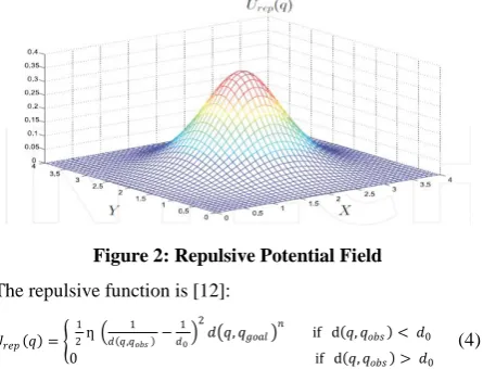
The repulsive force is inversely proportional to the distance from the obstacle. The repulsive potential results from the combination of the repulsive forces of all the obstacles. The equation of repulsive potential field is shown in Figure (2).
𝑈𝑟𝑒𝑝 𝑞 = 𝑈𝑖 𝑟𝑒𝑝𝑖 𝑞 (3)
Where Urepi(q) represents the repulsive potential generated by
[image:2.595.57.280.419.589.2]obstacle i, where i is no. of obstacles that influence the environment of robot
Figure 2: Repulsive Potential Field
The repulsive function is [12]:
𝑈𝑟𝑒𝑝 𝑞 = 1 2 ƞ
1 𝑑 𝑞,𝑞𝑜𝑏𝑠 −
1 𝑑0
2
𝑑 𝑞, 𝑞𝑔𝑜𝑎𝑙 𝑛 if d 𝑞, 𝑞𝑜𝑏𝑠 < 𝑑0
0 if d 𝑞, 𝑞𝑜𝑏𝑠 > 𝑑0
(4)
Where q is the robot position and qobs is the obstacle position.
d0 is the positive constant represents the distance of influence
of the obstacle, d(q,qobs) is the distance between the robot and
obstacle. ƞ is an adjustable constant represents the proportional coefficient of the repulsive potential filed function. The repulsive force is the negative gradient of this repulsive potential fields function.
𝐹𝑟𝑒𝑝 𝑞 = −∇𝑈𝑟𝑒𝑝 𝑞 = ƞ
1 𝑑 𝑞, 𝑞𝑜𝑏𝑠 −
1 𝑑0
(𝑞 − 𝑞𝑜𝑏𝑠)
𝑑3(𝑞 − 𝑞
𝑜𝑏𝑠) , if d 𝑞, 𝑞𝑜𝑏𝑠
< 𝑑0
0 , if d 𝑞, 𝑞𝑜𝑏𝑠 > 𝑑0
(5)
The total potential field is defined as the combination of attractive potential Uatt and a repulsive potential Urep. Then the
composition attractive potential with repulsive potential will
generate the total potential fields [13]. Then the total potential fields can be described by:
U 𝑞 = 𝑈𝑎𝑡𝑡 𝑞 + 𝑈𝑟𝑒𝑝 𝑞 (6)
The total force that applied to the mobile robot is obtained by the negative gradient of a total potential field which is the steepest descent direction for guiding robot to target point.
𝐹 𝑞 = −∇𝑈 𝑞 = − ∇𝑈𝑎𝑡𝑡− ∇𝑈𝑟𝑒𝑝 (7)
Where ∆U is the gradient vector of U at the robot position, the force that effected robot is defined as the sum of the two attractive and repulsive force vectors, Fatt and Frep,
respectively.
𝐹 𝑞 =𝐹𝑎𝑡𝑡(𝑞) + 𝐹𝑟𝑒𝑝(𝑞) (8)
4.
MOTION CONTROL
In this paper, PID control is considered as a motion controller for controlling movement of mobile robot. PID control is one of the classical control methods and widely used in the industrial applications. The majority of industrial control system still uses PID controllers for many applications in most systems. In the PID control, the difference between the set point or desired input value ref(t) and the actual output y(t) is represented by the e(t) error signal given by [e(t) = ref(t) – y(t)], This signal is applied to PID controller to get control signal u(t) as follows [14]:
𝑢 𝑡 = 𝐾𝑝𝑒 𝑡 + 𝐾𝑑𝑑𝑒 (𝑡)𝑑𝑡 + 𝐾𝑖 𝑒(𝑡)0𝑡 𝑑𝑡
(9)
KP = proportional gain , Ki = integral gain and Kd= derivative gain.
PID parameters (Kp, Ki and Kd) should be chosen carefully to
obtain fast rise time, no steady state error and smaller overshoot. In this paper PID controller parameters are tuned using Particle swarm optimization Algorithm “PSO” to get optimal response of PID Controller. The block diagram of control system for mobile robot with two PID controllers is shown in Figure (3).
Figure 3: Block diagram of control system with two PID controllers
5.
OPTIMIZATION OF PID
CONTROLLER BY PARTICLE SWARM
OPTIMIZATION ALGORITHM
[image:2.595.318.545.493.592.2]best solution and that solution called pbest. Particle swarm optimizer is also keeping track another value called the best value that get by particle in the neighbors of the particle. This location is called lbest. When one of particles takes all the population as its topological neighbors, the best value is a global best and it is named gbest [16]. The PSO algorithm is used to find the optimal parameters for the two PID controllers, one for controlling velocity and another for controlling angle of mobile robot. Figure (4) shows the block diagram of PID-PSO controller for the mobile robot.
Figure 4: the block diagram of optimal PID controller for the mobile robot.
The PSO algorithm will be used to tune two PID controllers by searching for their optimal value in the six dimensional search space [i.e. KP1,KI1,KD1, KP2,KI2,KD2], three dimensions
specified for first controller (velocity controller) and another three dimensions for second controller (angle controller), for each controller there are three parameter to be tuned. By doing several experiments using different values for population size and number of iterations, it is observed that the following parameters values of PSO algorithm shown in Table (1) yield acceptable parameters for PID controllers to give a good performance to control the movement of mobile robot.
Table (1): PSO parameters
Size of the swarm 100
Maximum iteration number 200
Dimension 6
PSO parameter c1 2
PSO parameter c2 2
Wmax 0.9
Wmin 0.3
Mean Square Error MSE criterion has been used as a fitness function to evaluate the performance of the system to compute the acceptable parameters by PSO algorithm. The formula of MES error is shown below:
𝑴𝑺𝑬𝒕𝒐𝒕𝒂𝒍= 𝟏𝒏 𝒆𝒏𝒌 𝜽(𝒌) 𝟐 + 𝟏
𝒏 𝒆𝒗(𝒌) 𝟐 𝒏
𝒌 (10)
n: represents number of samples, k: sample time. The parameters in the Table 2 give the best (lowest) MSE in order to build the PID controllers
Table (2): PID controller parameters
Parameters for PID controller to control velocity
Parameters for PID controller to control angle
KP1 KI1 KD1 KP2 KI2 KD2
110.44 50.24 1.0022 60 100.59 2.213
6.
LIMITATIONS AND PROPOSED
SOLUTIONS
Artificial Potential Field algorithm suffers from some drawbacks in implementing it for real time applications. The local minima problem is the most common problem, a local minima problem occurs when sum of all forces is zero. The most three conditions in which local minima occur are:
[image:3.595.60.286.182.316.2](1) When robot, obstacle and target are set on the same line and the obstacle is at the middle of the robot and the target [17]. The diagram in the Figure (5) below shows this case.
Figure 5: Robot, obstacle and target are located on the same line
(2) When the target is within the effected region of an obstacle such that the repulsive force of the obstacle will push the robot away from the goal point. The problem in the third condition is known as “Goals non-reachable with obstacle nearby” [18]. Diagram in the Figure (6) below illustrates this case.
Figure 6: Goals non-reachable with obstacle nearby problem
The drawbacks of traditional method can be solved by modifying repulsive potential functions.
6.1
Modified Repulsive Potential Field
Function
[image:3.595.331.527.301.366.2] [image:3.595.339.515.477.559.2] [image:3.595.56.279.495.660.2]minimum is at the target position [12]. The redefinition of repulsive potential function can be described by
𝑈𝑟𝑒𝑝 𝑞 =
1 2 ƞ
1 𝑑𝑞,𝑞𝑜𝑏𝑠 −
1 𝑑0
2
𝑑 𝒒, 𝒒𝒈𝒐𝒂𝒍𝒏, if d𝑞, 𝑞𝑜𝑏𝑠 <𝑑0
0 if d𝑞, 𝑞𝑜𝑏𝑠 > 𝑑0
(11)
where d(q,qobs)n represents the distance between the robot and
the goal , where n is a real number greater than 0 . So now when the mobile robot is close to the goal, the attractive potential field is reducing; the repulsive potential field is also reducing accordingly, until the robot reaches the goal point, then the attractive and repulsive field reduced to 0. The repulsive force is the negative gradient of repulsive potential fields function, and the composition of repulsive forces can be decomposed into two forces [17]. The composition of repulsive forces Frep can be described by:
𝐹𝑟𝑒𝑝= −∇𝑈𝑟𝑒𝑝𝑞 = 0𝐹 if d𝑟𝑒𝑝1+ 𝐹𝑟𝑒𝑝2 if d𝑞, 𝑞𝑞, 𝑞𝑜𝑏𝑠 <𝑑0
𝑜𝑏𝑠 >𝑑0 (12)
Both Frep1 and Frep2 are the decomposition of Frep , Frep1 and
Frep2 can be described as below:
𝐹𝑟𝑒𝑝 1 𝑞 = ƞ
1 𝑑𝑞,𝑞𝑜𝑏𝑠 −
1 𝑑0
𝑑 𝑞,𝑞𝑔𝑜𝑎𝑙 𝑛
𝑑(𝑞−𝑞𝑜𝑏𝑠)2
(13)
𝐹𝑟𝑒𝑝 2 𝑞 =−ƞ
𝑛 2
1 𝑑𝑞,𝑞𝑜𝑏𝑠 −
1
𝑑0 𝑑 𝑞, 𝑞𝑔𝑜𝑎𝑙
𝑛−1
(14)
Where Frep1 and Frep2 are two components of Frep. The
direction of Frep1 points to the mobile robot from the point,
which is closest to the robot. The direction of Frep2 points to
the goal from the mobile robot.
6.2 Optimization the Parameters of
Artificial Potential Field Method
In this section the PSO algorithm will be used to tune the parameters of artificial potential field parameters (i.e. ζ: proportional coefficient of the attractive potential filed function and ƞ: proportional coefficient of the repulsive potential filed function) to increase the efficiency of artificial potential field method. The two parameters will be tuned in the same search space of PID controller in section 5. So the number of parameters that will be tuned by PSO algorithm are eight parameters [KP1,KI1,KD1,KP2,KI2,KD2,Kζ,KƞKƞ]. Same parameters values of PSO algorithm shown in Table (1) will be used in this section. Table (3) illustrates gain parameters that yielded from PSO algorithm for PID controllers and APF.
Table (3): PID and APF parameters
Parameters for PID controller to Control velocity
Parameters for PID controller to Control Angle
ζ ƞ
KP1= 110.44
KI1= 50.2
KD1= 1.0022
KP2 =60
KI2= 100.59
KD2= 2.21
0.5 0.0047
7.
SIMULATION RESULTS
7.1 First Environment
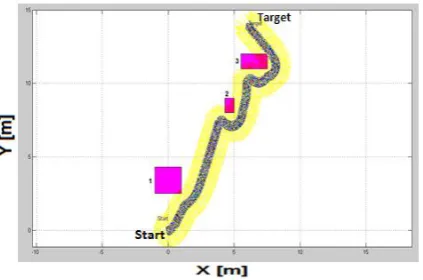
[image:4.595.319.531.72.212.2]Figure (7) illustrates the simulation of mobile robot navigation by using “Modified-Optimized Potential Field Method” as a path planning algorithm. In this environment the mobile robot moves from start point (0,0) to target point (6,14) where three static obstacles in the environment.
Figure 7: mobile robot movement in first environment.
7.2 Second Environment
[image:4.595.318.531.319.458.2]Figure (8) illustrates the simulation of mobile robot navigation by using “Modified-Optimized Potential Field Method” as a path planning algorithm in the second environment. In this environment the mobile robot moves from start point (0,0) to target point (14,16) where many static obstacles with different sizes speared in the environment.
Figure 8: Mobile robot movement in second environment.
Table (4) shows the elapsed time (sec) and path long (m) of mobile robot in the environments before and after optimization by PSO algorithm.
Table (4): Elapsed time and path long results
Before Optimization
First Environment
Second Environment
Total Elapsed Time(sec) to reach goal
3.8 4.16
Distance of path (m) 21.9 25
After Optimization
First Environment
Second Environment
Total Elapsed Time(sec) to reach goal
3.6 4.12
[image:4.595.311.545.535.723.2] [image:4.595.55.281.576.672.2]8.
CONCLUSION
A modification for the functions of potential field method can solve the problem of local minima and enable mobile robot to navigate in the environment from start point to the goal point while avoiding obstacles. The scaling parameters of the attractive and repulsive potential functions (ζ and ƞ) determine the relative intensity of the attractive force and the repulsive force, so an optimization for these two parameters by using Particle Swarm Optimization (PSO) method gives the optimal motion and grantee fast and smooth robot path. The simulation in matlab program shows that modified-optimized potential field method enables mobile robot to navigate in environment from start point to the target with less time and short path. Actually in the future work the potential field method need to combine with an intelligent technique (for example Fuzzy logic) to produce a robust method for path planning of mobile robot to navigate in complex and dynamic environment.
9.
REFERENCES
[1] Shahab Sheikh-Bahaei, ''Discrete Event Modeling Simulation and Control with Application to Sensor Based Intelligent Mobile Robotics'', M.Sc. Thesis, Electrical Engineering, The University of New Mexico, December, 2003.
[2] Hui Miao, “Robot Path Planning in Dynamic Environments Using a Simulated Annealing Based Approach”, M.Sc. Thesis, Queensland University of Technology, March 2009
[3] Luciano C. A. Pimenta1, Alexandre R. Fonseca, and Guilherme A. S. Pereira, “On Computing Complex Navigation Functions”, Proceedings of the 2005 IEEE International Conference on Robotics and Automation Barcelona, Spain, April 2005
[4] Khatib O.,"Real-Time Obstacle Avoidance for Manipulators and Mobile Robots", International Journal of Robotic Research, vol. 5, pp. 90-98, 1986.
[5] Liu Chengqing, Marcelo HAng Jr, Hariharan Krishnan and Lim Ser Yong, “Virtual Obstacle Concept for Local-minimum-recovery in Potential-field Based Navigation”, Proceedings of the 2000 IEEE International Conference on Robotics & Automation San Francisco, CA • April 2000
[6] P. Vadakkepat, K. C. Tan, and W. Ming‐Liang, “Evolutionary Artificial Potential Fields and their Application in Real Time Robot Path Planning”, Congress on Evolutionary Computation (2000) 1256 – 263.
[7] Ge, S. S. and Cui, Y. J., "Dynamic Motion Planning for Mobile Robots Using Potential Field Method", Autonomous Robots, vol. 13, pp. 207-222, 2002.
[8] Ge, S. S. and Cui, Y. J., "New Potential Functions for Mobile Robot Path Planning", IEEE Transactions on Robotics and Automation, vol. 16, pp. 615-620, 2002.
[9] Volpe, R. and Khosla, P., "Manipulator Control with Superquadric Artificial Potential Functions: Theory and Experiments", IEEE Transactions on Systems, Man and Cybernetics, vol. 20, pp. 1423-1436, 1990.
[10]Lee, L.-F., "Decentralized Motion Planning Within an Artificial Potential Framework (APF) for Cooperative Payload Transport by Multi-Robot Collectives", Mechanical & Aerospace Engineering, State University of New York at Buffalo, NY, Buffalo, 2004.
[11]Miguel A. Padilla Castaneda, Jesus Savage, Adalberto Hernandez and Fernando Arambula Cosío, “Local Autonomous Robot Navigation Using Potential Fields”, Xing-Jian Jing (Ed.), ISBN: 978-953-7619-01-5, InTech.
[12]Jinchao Gue, Yu Gao and Guangzhao Cui, “Path planning of mobile Robot base on Improved Potential Field”, Information Technology Journal 12(11) 2013
[13]Guanghui Li, Atsushi Yamashita and Hajime Asama Yusuke Tamura, “An Efficient Improved Artificial Potential Field Based Regression Search Method for Robot Path Planning”, Proceedings of the 2000 IEEE International Conference on Robotics & AutomationSan Francisco, CA • April 2000
[14]Vipul B. Patel , Virendra singh and Ravi H.Acharya, “Design of FPGA-based All Digital PID Controller for Dynamic Systems”, International Journal of Advanced Research in Electrical, Electronics and Instrumentation Engineering Vol. 1, Issue 2, August 2012
[15]M. Gupta, L. Behera and K. S. Venkatesh, “PSO based modeling of Takagi-Sugeno fuzzy motion controller for dynamic object tracking with mobile platform”, Proceedings of IEEE the International Multiconference on Computer Science and Information Technology, Vol. (5), pp. 37–43, Poland, 2010
[16]K. Ramanathan , V.M. Periasamy , M. Pushpavanam and U. Natarajan, “ Particle Swarm Optimisation of hardness in nickel diamond electro composites”, International Scientific Journal 2009 vol. 1 issue 4 232-236
[17]Su Weijun, Meng Rui and Yu Chongchong, “A Study on Soccer Robot Path Planning with Fuzzy Artificial Potential Field”, Proceedings of the 2010 International Conference on Computing, Control and Industrial Engineering (CCIE), vol.1 ,pp.386-390 (2010)