Munich Personal RePEc Archive
Forecasting spot electricity prices: A
comparison of parametric and
semiparametric time series models
Weron, Rafal and Misiorek, Adam
Hugo Steinhaus Center, Wroclaw University of Technology
10 June 2008
Online at
https://mpra.ub.uni-muenchen.de/10428/
Forecasting spot electricity prices: A comparison of
parametric and semiparametric time series models
Rafa l Weron
a, Adam Misiorek
ba
Hugo Steinhaus Center, Institute of Mathematics and Computer Science, Wroc law University of Technology, Wroc law, Poland
bSantander Consumer Bank S.A., Wroc law, Poland
Abstract
This empirical paper compares the accuracy of 12 time series methods for short-term (day-ahead) spot price forecasting in auction-type electricity markets. The methods considered in-clude standard autoregression (AR) models, their extensions – spike preprocessed, threshold and semiparametric autoregressions (i.e. AR models with nonparametric innovations), as well as, mean-reverting jump diffusions. The methods are compared using a time series of hourly spot prices and syswide loads for California and a series of hourly spot prices and air tem-peratures for the Nordic market. We find evidence that (i) models with system load as the exogenous variable generally perform better than pure price models, while this is not necessarily the case when air temperature is considered as the exogenous variable, and that (ii) semipara-metric models generally lead to better point and interval forecasts than their competitors, more importantly, they have the potential to perform well under diverse market conditions.
Key words: Electricity market, Price forecast, Autoregressive model, Nonparametric maximum likelihood, Interval forecast, Conditional coverage.
1. Introduction
Over the past two decades a number of countries around the world have decided to take the path of power market liberalization. This process, based upon the idea of separation of services and infrastructures, has changed the power industry from the centralized and vertically integrated structure to an open, competitive market environment (Kirschen and Strbac, 2004, Weron, 2006). Electricity is now a commodity that can be bought and sold at market rates. However, it is a very specific commodity. Electricity demand is weather
Email addresses:rafal.weron@pwr.wroc.pl(Rafa l Weron),adam.misiorek@santanderconsumer.pl (Adam Misiorek).
and business cycle dependent. At the same time it is price inelastic, at least over short time horizons, as most consumers are unaware of or indifferent to the current price of electricity. On the other hand, electricity cannot be stored economically while power system stability requires a constant balance between production and consumption. These factors lead to extreme price volatility (up to 50% on the daily scale) and to one of the most pronounced features of electricity markets – the abrupt and generally unanticipated extreme changes in the spot prices known as spikes, see the top panels in Figures 1 and 2.
Like most other commodities, electricity is traded both on regulated markets (power exchanges or power pools) and over-the-counter (through so-called bilateral contracts). In the power exchange, wholesale buyers and sellers take part in a (uniform price) auction and submit their bids in terms of prices and quantities. The spot price, i.e. the set of clearing prices for the 24 hours (or 48 half-hour intervals in some markets) of the next day, is calculated as the intersection between the aggregated supply and demand curves.
This paper is concerned with short-term spot price forecasting (STPF) in the uniform price auction setting. Predictions of hourly spot prices are made for up to a week ahead, however, usually the focus is on day-ahead forecasts only. In this empirical study we follow the ‘standard’ testing scheme: to compute price forecasts for all 24 hours of a given day, the data available to all procedures includes price and load (or other fundamental variable) his-torical data up to hour 24 of the previous day plus day-ahead predictions of the fundamental variable for the 24 hours of that day. An assumption is made that only publicly available information is used to predict spot prices, i.e. generation constraints, line capacity limits or other power system variables are not considered. Note, that market practice differs from this ‘standard’ testing scheme in that it uses historical data only up to a certain morning hour (9-11 a.m.) of the previous day, and not hour 24, as the bids have to be submitted around mid-day, not after midnight.
There are many approaches to modeling and forecasting spot electricity prices, but only some of them are well suited for STPF (for a review we refer to Weron, 2006). Time series models constitute one of the most important groups. Generally, specifications where each hour of the day is modeled separately present better forecasting properties than specifica-tions common for all hours (Cuaresma et al., 2004). However, both approaches are equally popular. Apart from basic AR and ARMA specifications, a whole range of alternative mod-els have been proposed. The list includes ARIMA and seasonal ARIMA modmod-els (Contreras et al., 2003, Zhou et al., 2006), autoregressions with heteroskedastic (Garcia et al., 2005) or heavy-tailed (Weron, 2008) innovations, AR models with exogenous (fundamental) vari-ables – ‘dynamic regression’ (or ARX) and ‘transfer function’ (or ARMAX) models (Conejo et al., 2005), vector autoregressions with exogenous effects (Panagiotelis and Smith, 2008), threshold AR and ARX models (Misiorek et al., 2006), regime-switching regressions with fundamental variables (Karakatsani and Bunn, 2008) and mean-reverting jump diffusions (Knittel and Roberts, 2005).
and without exogenous variables. The empirical analysis is conducted for two markets and under various market conditions.
The paper is structured as follows. In Section 2 we describe the datasets. Next, in Section 3 we introduce the models and calibration details. Section 4 provides point and interval forecasting results for the studied models. Both, unconditional and conditional coverage of the actual spot price by the model implied prediction intervals is statistically tested. Finally, Section 5 concludes.
2. The data
The datasets used in this empirical study include market data from California (1999-2000) and Nord Pool (1998-1999, 2003-2004). Such a range of data allows for a thorough evaluation of the models under different conditions. The California market is chosen for two reasons: it offers freely accessible, high quality data and exhibits variable market behavior with extreme spikes. The Nordic market, on the other hand, is a less volatile one with majority of generation coming from hydro production. Consequently, not only the demand but also the supply is largely weather dependent. The level of the water reservoirs in Scandinavia translates onto the level and behavior of electricity prices (Weron, 2008). Two periods are selected for the analysis: one with high water reservoir levels (1998-1999), i.e. above the 13-year median, and one with low levels (2003-2004).
2.1. California (1999-2000)
This dataset includes hourly market clearing prices from the California Power Exchange (CalPX), hourly system-wide loads in the California power system and their day-ahead fore-casts published by the California Independent System Operator (CAISO). The time series were constructed using data downloaded from the UCEI institute (www.ucei.berkeley.edu) and CAISO (oasis.caiso.com) websites and preprocessed to account for missing values and changes to/from the daylight saving time; for details see Section 4.3.7 in Weron (2006) and the MFE Toolbox (www.im.pwr.wroc.pl/˜rweron/MFE.html).
The time series used in this study are depicted in Figure 1. The day-ahead load forecasts are indistinguishable from the actual loads at this resolution; only the latter are plotted. We used the data from the (roughly) 9-month period July 5, 1999 – April 2, 2000 only for calibration. The next ten weeks (April 3 – June 11, 2000) were used for out-of-sample testing. For every day in the out-of-sample test period we ran a day-ahead prediction, forecasting the 24 hourly prices. We applied an adaptive scheme, i.e. instead of using a single parameter set for the whole test sample, for every day (and hour) in the out-of-sample period we calibrated the models, given their structure, to the available data. At each estimation step the ending date of the calibration sample (but not the starting date) was shifted by one day:
– to forecast prices for the 24 hours of April 3 we used prices, loads and load forecasts from the period July 5, 1999 – April 2, 2000,
– to forecast prices for the 24 hours of April 4 we used prices, loads and load forecasts from the period July 5, 1999 – April 3, 2000, etc.
Note, that the day-ahead load forecasts published by CAISO on dayT actually concern the 24 hours of dayT+ 1.
Jul 5, 1999 Jan 1, 2000 Apr 3, 2000 Jun 11, 2000 0
100 200 300 400 500
Price [USD/MWh]
Hours [Jul 5, 1999 − Jun 11, 2000]
← Calibration start Forecast
(weeks 1−10)
Jul 5, 1999 15 Jan 1, 2000 Apr 3, 2000 Jun 11, 2000 20
25 30 35 40 45 50
Load [GW]
Hours [Jul 5, 1999 − Jun 11, 2000]
← Calibration start Forecast
[image:5.595.146.466.127.373.2](weeks 1−10)
Fig. 1. Hourly system prices (top) and hourly system loads (bottom) in California for the period July 5, 1999 – June 11, 2000. The out-of-sample ten week test period (Apr. 3 – June 11, 2000) is marked by a rectangle.
procedure resulted in generally worse forecasts. For instance, for the AR/ARX models (see Section 3.2) the rolling window scheme led to better predictions (in terms of the WMAE measure, see Section 4) only for one (#7) out of ten weeks of the out-of-sample period.
Finally, let us mention that the logarithms of loads (or load forecasts) were used as the exogenous (fundamental) variable in the time series models for the log-prices. This selection was motivated by the approximately linear dependence between these two variables. In the studied period the Pearson correlation between log-prices and log-loads is positive (ρ= 0.64) and significant (p-value ≈0; null of no correlation). This relationship is not surprising if we recall, that as a result of the supply stack structure, load fluctuations translate into variations in electricity prices, especially on the hourly time scale.
2.2. Nord Pool (1998-1999)
This dataset comprises hourly Nord Pool market clearing prices and hourly temperatures from the years 1998-1999. The time series were constructed using data published by the Nordic power exchange Nord Pool (www.nordpool.com) and the Swedish Meteorological and Hydrological Institute (www.smhi.se). They were preprocessed in a way similar to that of the California dataset.
Apr 6, 19980 Jan 1, 1999 Dec 5, 1999 100
200 300 400 500
← Calibration start II V VIII XI
Hours [Apr 6, 1998 − Dec 5, 1999]
Price [NOK/MWh]
Apr 6, 1998 Jan 1, 1999 Dec 5, 1999
−10 0 10 20
30 ← Calibration start II V VIII XI
Hours [Apr 6, 1998 − Dec 5, 1999]
Temperature [
[image:6.595.147.466.129.374.2]oC]
Fig. 2. Hourly system prices (top) and hourly air temperatures (bottom) in Nord Pool area for the period April 6, 1998 – December 5, 1999. The four out-of-sample five-week test periods are marked by rectangles. They roughly correspond to calendar months of February (II: Feb. 1 – Mar. 7, 1999), May (V: Apr. 26 – May 30, 1999), August (VIII: Aug. 2 – Sept. 5, 1999) and November (XI: Nov. 1 – Dec. 5, 1999).
The dependence between log-prices and temperatures is not as strong as the load-price relationship in California, nevertheless they are moderately anticorrelated, i.e. low tempera-tures in Scandinavia imply high electricity prices at Nord Pool and vice versa (see Figure 2). In the studied period the Pearson correlation between log-prices and temperatures is nega-tive (ρ=−0.47) and significant (p-value≈0; null of no correlation). We have to note also, that the ‘hourly air temperature’ is in fact a proxy for the air temperature in the whole Nord Pool region. It is calculated as an arithmetic average of the hourly air temperatures of six Scandinavian cities/locations (Bergen, Helsinki, Malm¨o, Stockholm, Oslo and Trondheim). Like for California, an adaptive scheme and a relatively long calibration sample was used. It started on April 6, 1998 and ended on the day directly preceding the 24 hours for which the price was to be predicted. Four five-week periods were selected for model evaluation, see Figure 2. This choice of the out-of-sample test periods was motivated by a desire to evaluate the models under different conditions, corresponding to the four seasons of the year.
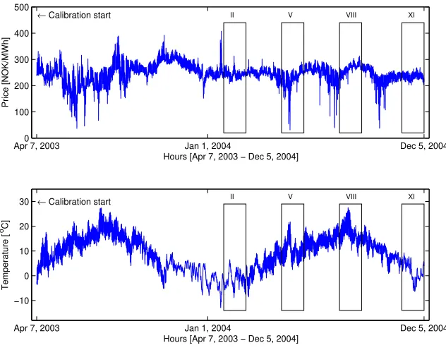
2.3. Nord Pool (2003-2004)
This dataset was constructed analogously to the Nord Pool (1998-1999) sample. The Pearson correlation between log-prices and temperatures (ρ=−0.06) is much weaker than in the 1998-1999 dataset (but still highly significant:p-value ≈0; null of no correlation). This change is mostly due to the fact that in 2003-2004 water reservoir levels in Scandinavia were low and the spot price was generated more by lack of supply than demand.
Apr 7, 20030 Jan 1, 2004 Dec 5, 2004 100
200 300 400 500
← Calibration start II V VIII XI
Hours [Apr 7, 2003 − Dec 5, 2004]
Price [NOK/MWh]
Apr 7, 2003 Jan 1, 2004 Dec 5, 2004
−10 0 10 20
30 ← Calibration start II V VIII XI
Hours [Apr 7, 2003 − Dec 5, 2004]
Temperature [
[image:7.595.148.464.130.378.2]oC]
Fig. 3. Hourly system prices (top) and hourly air temperatures (bottom) in Nord Pool area for the period April 7, 2003 – December 5, 2004. The four out-of-sample five-week test periods are marked by rectangles. They roughly correspond to calendar months of February (II: Jan. 26 – Feb. 29, 2004), May (V: Apr. 26 – May 30, 2004), August (VIII: July 26 – Aug. 29, 2004) and November (XI: Nov. 1 – Dec. 5, 2004).
sample was used. It started on April 7, 2003 and ended on the day directly preceding the 24 hours for which the price was to be predicted. Like for the Nord Pool (1998-1999) dataset, four five-week periods were selected for model evaluation, see Figure 3.
3. The models
3.1. Preliminaries
The logarithmic transformation was applied to price,pt= log(Pt), and load,zt= log(Zt),
data to attain a more stable variance (but not to temperatures). Furthermore, the mean price and the median load were removed to center the data around zero. Removing the mean load resulted in worse forecasts, perhaps, due to the very distinct and regular asymmetric weekly structure with the five weekday values lying in the high-load region and the two weekend values – in the low-load region.
Since each hour displays a rather distinct price profile reflecting the daily variation of demand, costs and operational constraints the modeling was implemented separately across the hours, leading to 24 sets of parameters (for each day the forecasting exercise was per-formed). This approach was also inspired by the extensive research on demand forecast-ing, which has generally favored the multi-model specification for short-term predictions (Bunn, 2000, Shahidehpour et al., 2002, Weron, 2006).
the models and (ii) daily dummy variables. The log-price pt was made dependent on the
log-prices for the same hour on the previous two days, and the previous week, as well as the minimum of all prices on the previous day. The latter created the desired link between bidding and price signals from the entire day. Other functions (maximum, mean, median) have been tried as well, but they have led to worse forecasts.
Furthermore, three dummy variables (for Monday, Saturday and Sunday) were consid-ered to differentiate between the two weekend days, the first working day of the week and the remaining business days. This particular choice of the dummies was motivated by the significance of the dummy coefficients for particular days (we tested the null hypothesis that a particular coefficient is not significantly different from zero; see also the last paragraph in Section 3.2). For all three datasets – California and two Nord Pool periods, the Monday dummy was significant most often (for nearly 70% of the hours thep-values were less than 0.05), followed by Saturday and Sunday.
Finally, recall that all models were estimated using an adaptive scheme. Instead of using a single model for the whole test sample, for every day (and hour) in the test period we reestimated the model coefficients (given its structure; see below) to the previous values of prices (and exogenous variables) and obtained a predicted value for that day (and hour). The model structures remained the same throughout the forecasting exercise (they were the same for all three datasets), only the coefficients were recalibrated every day (and hour).
3.2. Basic autoregressive models
In our models we used only one exogenous variable. For California it was (the logarithm of) the hourly system-wide load. At lag 0 the CAISO day-ahead load forecast for a given hour was used, while for larger lags the actual system load was used. Interestingly, the best models turned out to be the ones with only lag 0 dependence. Using the actual load at lag 0, in general, did not improve the forecasts either. This phenomenon can be explained by the fact that the prices are an outcome of the bids, which in turn are placed with the knowledge of load forecasts but not actual future loads. For the Nord Pool datasets the hourly air temperature was the only exogenous variable. At lag 0 the actual temperatures observed on that day were used (day-ahead hourly temperature forecasts were not available to us).
The basic autoregressive model structure used in this study is given by the following formula (denoted later in the text asARX):
pt=φ1pt−24+φ2pt−48+φ3pt−168+φ4mpt+
+ψ1zt+d1DM on+d2DSat+d3DSun+εt. (1)
The lagged log-prices pt−24, pt−48 and pt−168 account for the autoregressive effects of the
previous days (the same hour yesterday, two days ago and one week ago), whilemptcreates
the link between bidding and price signals from the entire previous day (it is the minimum of the previous day’s 24 hourly log-prices). The variableztrefers to the log-load forecast (for
the California power market) or actual temperature (for Nord Pool). The three dummy vari-ables –DM on,DSatandDSun (for Monday, Saturday and Sunday, respectively) – account
for the weekly seasonality. Finally, the εt’s are assumed to be independent and identically
distributed (i.i.d.) with zero mean and finite variance (e.g. Gaussian white noise). Restrict-ing the parameter ψ1 = 0 yields the AR model. Model parameters can be estimated by
This particular choice of model variables (pt−24, pt−48, pt−168, mpt, zt, DM on, DSat and DSun) was motivated by the significance of their coefficients. For the first weeks of all nine
out-of-sample test periods (one for California and four for each of the Nord Pool datasets; see Figures 1-3) we tested the null hypothesis that a particular coefficient is not significantly different from zero. The tested variables included: pt−24·i for i = 1, ...,6, pt−168·j for j =
1, ...,4, mpt = (max,min,mean,median), zt−24·k for k = 0,1, ...,7, andDxxx with xxx=
(Mon, Tue, Wed, Thu, Fri, Sat, Sun). The significance varied across the datasets and across time, but overall the above eight were the most influential variables. Hypothetically, the significance of the variables could be tested for each day and each hour of the test period. However, this procedure would be burdensome and we decided not to execute this option. Instead we used one common and on average optimal model structure for all datasets.
3.3. Spike preprocessed models
In the system identification context, infrequent and extreme observations pose a serious problem. A single outlier is capable of considerably changing the coefficients of a time series model. In our case, price spikes play the role of outliers. Unfortunately, defining an outlier (or a price spike) is subjective, and the decisions concerning how to identify them must be made on an individual basis. Also the decisions how to treat them. One solution could be to use a model which admits such extreme observations, another – to exclude them from the calibration sample. We will return to the former solution in Sections 3.4 and 3.5. Now let us concentrate on data preprocessing, with the objective of modifying the original observations in such a way as to make them more likely to come from a mean-reverting (autoregressive) spikeless process. We have to note, that this is quite a popular approach in the electrical engineering price forecasting literature (see e.g. Conejo et al., 2005, Contreras et al., 2003, Shahidehpour et al., 2002).
In time series modeling we cannot simply remove an observation, as this would change the temporal dependence structure. Instead we can substitute it with another, ‘less unusual’ value. This could be done in a number of ways. Weron (2006) tested three approaches and found a technique he called the ‘damping scheme’ to perform the best. In this scheme an upper limitT was set on the price (equal to the mean plus three standard deviations of the price in the calibration period). Then all pricesPt> T were set toPt=T+Tlog10(Pt/T).
Although we don’t believe that forecasters should ignore the unusual, extreme spiky prices, we have decided to compare the performance of this relatively popular approach to that of other time series specifications. The spike preprocessed models, denoted in the text as p-ARXand p-AR, also utilize formula (1), with the only difference that the data used for calibration is spike preprocessed using the damping scheme.
3.4. Regime switching models
Regime switching models come in handy whenever the assumption of a non-linear mech-anism switching between normal and excited states or regimes of the process is reasonable. In the context of this study, electricity price spikes can be very naturally interpreted as changes to the excited (spike) regime of the price process.
levelT. TheTARXspecification used in this study is a natural generalization of the ARX model defined by (1):
pt=φ1,ipt−24+φ2,ipt−48+φ3,ipt−168+φ4,impt+
+ψ1,izt+d1,iDM on+d2,iDSat+d3,iDSun+εt,i. (2)
where the subscriptican be 1 (for the base regime when vt≤T) or 2 (for the spike regime
when vt> T). Setting the coefficients ψ1,i = 0 gives rise to the TAR model. Building on
the simulation results of Weron (2006) we setT = 0 andvt equal to the difference in mean
prices for yesterday and eight days ago. Like for AR/ARX models, the parameters can be estimated by minimizing the FPE criterion.
3.5. Mean-reverting jump diffusions
Mean-reverting jump diffusion (MRJD) processes have provided the basic building block for electricity spot price dynamics since the very first modeling attempts in the 1990s (Johnson and Barz, 1999, Kaminski, 1997). Their popularity stems from the fact that they address the basic characteristics of electricity prices (mean reversion and spikes) and at the same time are tractable enough to allow for computing analytical pricing formulas for elec-tricity derivatives. MRJD models have been also used for forecasting hourly elecelec-tricity spot prices (Cuaresma et al., 2004, Knittel and Roberts, 2005) and volatility (Chan et al., 2008), though with moderate success.
A mean-reverting jump diffusion model is defined by a (continuous-time) stochastic dif-ferential equation that governs the dynamics of the price process:
dpt= (α−βpt)dt+σdWt+Jdqt. (3)
The Brownian motion Wt is responsible for small (proportional to σ) fluctuations around
the long-term mean α
β, while an independent compound Poisson (jump) processqtproduces
infrequent (with intensity λ) but large jumps of size J (here: Gaussian with mean µ and variance γ2). In this study it is reasonable to allow the intercept α to be a deterministic
function of time to account for the seasonality prevailing in electricity spot prices.
The problem of calibrating jump diffusion models is related to a more general one of estimating the parameters of continuous-time jump processes from discretely sampled data (for reviews and possible solutions see Cont and Tankov, 2003, Weron, 2006). Here we follow the approach of Ball and Torous (1983) and approximate the model with a mixture of normals. In this setting the price dynamics is discretized (dt → ∆t; for simplicity we let ∆t = 1) and λ is assumed to be small, so that the arrival rate for two jumps within one period is negligible. Then the Poisson process is well approximated by a simple binary probabilityλ∆t=λof a jump (and (1−λ)∆t= (1−λ) of no jump) and the MRJD model (3) can be written as an AR(1) process with the mean and variance of the (Gaussian) noise term being conditional on the arrival of a jump in a given time interval. More explicitly, the
MRJDXspecification used in this study is given by the following formula:
pt=φ1pt−24+ψ1zt+d1DM on+d2DSat+d3DSun+εt,i, (4)
where the subscriptican be 1 (if no jump occurred in this time period) or 2 (if there was a jump),εt,1∼N(0, σ2) andεt,2∼N(µ, σ2+γ2). Setting the coefficientψ1= 0 gives rise to
3.6. Semiparametric extensions
The motivation for using semiparametric models stems from the fact that a nonparametric kernel density estimator will generally yield a better fit to empirical data than any parametric distribution. If this is true then, perhaps, time series models would lead to more accurate predictions if no specific form for the distribution of innovations was assumed. To test this conjecture we evaluate four semiparametric models – with and without the exogenous variable and using two different estimation schemes.
Under the assumption of normality the least squares (LS) and maximum likelihood (ML) estimators coincide and both methods can be used to efficiently calibrate autoregressive-type models. If the error distribution is not normal but is assumed to be known (up to a finite number of parameters), ML methods are still applicable, but generally involve numerical maximization of the likelihood function. If we do not assume a parametric form for the error distribution we have to extend the ML principle to a nonparametric framework, where the error density will be estimated by a kernel density estimator. The key idea behind this principle is not new. It has been used in a regression setting by Hsieh and Manski (1987) and for ARMA models by Kreiss (1987); see also H¨ardle et al. (1997).
In the present study we will use two nonparametric estimators for autoregressive models analyzed by Cao et al. (2003): the iterated Hsieh-Manski estimator (IHM) and the smoothed nonparametric ML estimator (SN). The IHM estimator is an iterated version of an adaptive ML estimator for ordinary regression (Hsieh and Manski, 1987). It is computed as follows. First, an initial vector of parametersφb0is obtained using any standard estimator (LS, ML).
Then, the model residuals bε(φb0) = {εbt(φb0)}n
t=1, i.e. the differences between actual values
and model forecasts, are used to compute the Parzen-Rosenblatt kernel estimator of the error density:
b
fh(x,bε(φb0)) = 1 nh
n
X
t=1
K x−bεt(φb0) h
!
, (5)
where K is the kernel, h is the bandwidth and n is the sample size. The nonparametric Hsieh-Manski estimator is then computed by (numerically) maximizing the likelihood:
b
φHM = arg max
φ Lbh(φ,φb0) = arg maxφ n
Y
t=1 b
fh(bεt(φ),bε(φb0)). (6)
The iterated version of the estimator is obtained by repeating the above steps with the Hsieh-Manski estimatorφbHM as the initial estimator:
b
φIHM = arg max
φ Lbh(φ,φbHM). (7)
Cao et al. (2003) suggest that this iteration should be beneficial when the true distribution is far from normal. The ARX and AR models (see formula (1)) calibrated with the iterated Hsieh-Manski estimator are denoted in the text asIHMARXandIHMAR, respectively. There are many possible choices for the kernel K and the bandwidth h used in for-mula (5), see e.g. H¨ardle et al. (2004) and Silverman (1986). For the sake of simplicity we will use the Gaussian kernel (which is identical to the standard normal probability density function) as it allows to arrive at an explicit, applicable formula for bandwidth selection:
h= 1.06 min{σ,ˆ R/ˆ 1.34}n−1/5. Here ˆσis an estimator of the standard deviation and ˆRis the
h= 1.06ˆσn−1/5; for more optimal bandwidth choices consult Cao et al. (1993) or Jones et
al. (1996). It will give a bandwidth not too far from the optimum if the error distribution is not too different from the normal distribution, i.e. if it is unimodal, fairly symmetric and does not have very heavy tails.
The smoothed nonparametric ML estimator (SN) is constructed analogously to the Hsieh-Manski estimator with the only difference that the kernel estimator of the error density (5) is computed for the residuals implied by the current estimate ofφinstead of those implied by some preliminary estimatorφb0:
b
φSN = arg max
φ Lbh(φ, φ) = arg maxφ n
Y
t=1 b
fh(εbt(φ),bε(φ)). (8)
The ARX and AR models, see formula (1), calibrated with the smoothed nonparametric ML estimator are denoted in the text asSNARXand SNAR, respectively.
Note, that unlike for the IMH estimator no preliminary estimator of φis needed in this case. On the other hand, one is tempted with choosing a different bandwidthhfor each value ofφ at which the likelihood is evaluated. For the sake of parsimony, we have not executed this option. Readers interested in this possibility and the effect it may have on the results are referred to the simulation study of Cao et al. (2003).
To our best knowledge, there have been no attempts to apply these nonparametric tech-niques in short-term electricity price forecasting to date. Only Weron (2008) obtained some preliminary, though encouraging, results for an ARX model calibrated using the smoothed nonparametric ML estimator (8). It is exactly the aim of this study to evaluate such methods and compare their forecasting performance to that of other time series models.
4. Forecasting performance
The forecast accuracy was checked afterwards, once the true market prices were available. Originally we used both a linear and a quadratic error measure, but since the results were qualitatively very much alike we have decided to present the results only for the linear measure. The Weekly-weighted Mean Absolute Error (WMAE, also known as the Mean Weekly Error or MWE) was computed as:
WMAE = ¯1
P168
MAE = 1 168·P¯168
X168
h=1
Ph−Pˆh
, (9)
wherePhwas the actual price for hourh, ˆPhwas the predicted price for that hour (taken as
the expectation of the model predicted log-price ˆph) and ¯P168=1681 P168h=1Ph was the mean
price for a given week. If we write the term 1/P¯168 under the sum in (9), then WMAE can
be treated as a variant of the Mean Absolute Percentage Error (MAPE) withPh replaced
by ¯P168. This replacement allows to avoid the adverse effect of prices close to zero.
4.1. Point forecasts
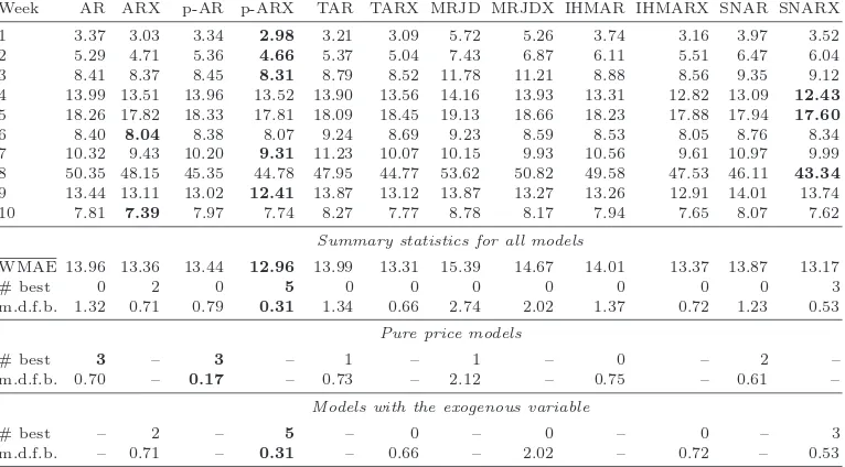
Table 1
The WMAE errors in percentage for all weeks of the California (1999-2000) test period. Best results in each row are emphasized in bold. Measures of fit are summarized in the bottom rows. They include the mean WMAE over all weeks (WMAE), the number of times a given model was best (# best) and the mean deviation from the best model in each week (m.d.f.b.). Notice that the results for the AR, ARX, TAR and TARX methods in this table were originally reported in Misiorek et al. (2006), while the results for the p-ARX model were originally reported in Weron (2006). They are re-produced here for comparison purpose.
Week AR ARX p-AR p-ARX TAR TARX MRJD MRJDX IHMAR IHMARX SNAR SNARX
1 3.37 3.03 3.34 2.98 3.21 3.09 5.72 5.26 3.74 3.16 3.97 3.52 2 5.29 4.71 5.36 4.66 5.37 5.04 7.43 6.87 6.11 5.51 6.47 6.04 3 8.41 8.37 8.45 8.31 8.79 8.52 11.78 11.21 8.88 8.56 9.35 9.12 4 13.99 13.51 13.96 13.52 13.90 13.56 14.16 13.93 13.31 12.82 13.09 12.43
5 18.26 17.82 18.33 17.81 18.09 18.45 19.13 18.66 18.23 17.88 17.94 17.60
6 8.40 8.04 8.38 8.07 9.24 8.69 9.23 8.59 8.53 8.05 8.76 8.34 7 10.32 9.43 10.20 9.31 11.23 10.07 10.15 9.93 10.56 9.61 10.97 9.99
8 50.35 48.15 45.35 44.78 47.95 44.77 53.62 50.82 49.58 47.53 46.11 43.34
9 13.44 13.11 13.02 12.41 13.87 13.12 13.87 13.27 13.26 12.91 14.01 13.74 10 7.81 7.39 7.97 7.74 8.27 7.77 8.78 8.17 7.94 7.65 8.07 7.62
Summary statistics for all models
WMAE 13.96 13.36 13.44 12.96 13.99 13.31 15.39 14.67 14.01 13.37 13.87 13.17
# best 0 2 0 5 0 0 0 0 0 0 0 3
m.d.f.b. 1.32 0.71 0.79 0.31 1.34 0.66 2.74 2.02 1.37 0.72 1.23 0.53
Pure price models
# best 3 – 3 – 1 – 1 – 0 – 2 –
m.d.f.b. 0.70 – 0.17 – 0.73 – 2.12 – 0.75 – 0.61 –
Models with the exogenous variable
# best – 2 – 5 – 0 – 0 – 0 – 3
m.d.f.b. – 0.71 – 0.31 – 0.66 – 2.02 – 0.72 – 0.53
gives indication which approach is the closest to the ‘optimal model’ composed of the best performing model in each week. It is defined as
m.d.f.b. = 1
T
T
X
t=1
(Ei,t−Ebest model,t), (10)
whereiranges over all evaluated models (i.e.i= 12 ori= 6),T is the number of weeks in the sample (10 for California, 20 for Nord Pool) andE is the WMAE error measure.
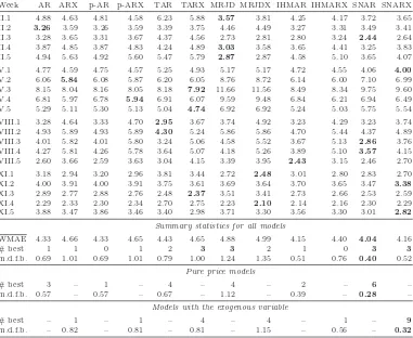
Table 2
The WMAE errors in percentage for all weeks of the Nord Pool (1998-1999) test period. Best results in each row are emphasized in bold. Like in Table 1, measures of fit are summarized in the bottom rows.
Week AR ARX p-AR p-ARX TAR TARX MRJD MRJDX IHMAR IHMARX SNAR SNARX
II.1 4.88 4.63 4.81 4.58 6.23 5.88 3.57 3.81 4.25 4.17 3.72 3.65 II.2 3.26 3.59 3.26 3.59 3.39 3.75 4.46 4.49 3.27 3.31 3.49 3.41 II.3 3.28 3.65 3.31 3.67 4.37 4.56 2.73 2.81 2.80 3.24 2.44 2.64 II.4 3.87 4.85 3.87 4.83 4.24 4.89 3.03 3.58 3.65 4.41 3.25 3.83 II.5 4.94 5.63 4.92 5.60 5.47 5.79 2.87 2.87 4.58 5.10 3.65 4.07
V.1 4.77 4.59 4.75 4.57 5.25 4.93 5.17 5.17 4.72 4.55 4.06 4.00
V.2 6.06 5.84 6.08 5.87 6.20 6.05 8.76 8.72 6.14 6.00 7.10 6.99
V.3 8.15 8.04 8.16 8.05 8.18 7.92 11.66 11.56 8.49 8.34 9.75 9.60 V.4 6.81 5.97 6.78 5.94 6.91 6.07 9.59 9.48 6.84 6.21 6.94 6.49 V.5 5.29 5.11 5.30 5.13 5.04 4.74 6.92 6.92 5.24 5.03 5.75 5.54
VIII.1 3.28 4.64 3.33 4.70 2.95 3.67 3.74 4.92 3.23 4.29 3.23 3.74 VIII.2 4.93 5.89 4.93 5.89 4.30 5.24 5.86 5.86 4.70 5.44 4.37 4.89 VIII.3 4.01 5.82 4.01 5.80 3.24 5.06 4.58 5.52 3.67 5.13 2.86 3.76 VIII.4 4.27 5.81 4.26 5.78 3.64 5.07 4.18 5.26 3.89 5.10 3.57 4.15 VIII.5 2.60 3.66 2.59 3.63 3.04 4.15 3.39 3.95 2.43 3.15 2.46 2.70
XI.1 3.18 2.94 3.20 2.96 3.81 3.44 2.72 2.48 3.01 2.80 2.83 2.70
XI.2 4.00 3.91 4.00 3.91 3.75 3.61 3.69 3.64 3.70 3.65 3.47 3.38
XI.3 2.89 2.77 2.88 2.76 2.48 2.37 3.51 3.41 2.73 2.66 2.53 2.59 XI.4 2.29 2.33 2.30 2.34 2.70 2.75 2.23 2.10 2.14 2.16 2.30 2.29 XI.5 3.88 3.47 3.86 3.46 3.40 2.98 3.71 3.30 3.56 3.30 3.01 2.82
Summary statistics for all models
WMAE 4.33 4.66 4.33 4.65 4.43 4.65 4.88 4.99 4.15 4.40 4.04 4.16
# best 1 1 0 1 2 3 3 2 1 0 3 3
m.d.f.b. 0.69 1.01 0.69 1.01 0.79 1.00 1.24 1.35 0.51 0.76 0.40 0.52
Pure price models
# best 3 – 1 – 4 – 4 – 2 – 6 –
m.d.f.b. 0.57 – 0.57 – 0.67 – 1.12 – 0.39 – 0.28 –
Models with the exogenous variable
# best – 1 – 1 – 4 – 4 – 1 – 9
m.d.f.b. – 0.82 – 0.81 – 0.81 – 1.15 – 0.56 – 0.32
Note, that the quadratic error measure (Root Mean Square Error for weekly samples) leads to slightly different conclusions for this dataset. The AR/ARX and IHMAR/IHMARX models perform very well on average (m.d.f.b. values) but rarely beat all the other com-petitors, the SNARX/SNAR models come in next. The spike preprocessed models still have the highest number of best forecasts, but on average fail badly due to the extremely poor performance in the 8th week. SNARX/SNAR are the only models that behave relatively well with regard to both error measures.
The WMAE errors for the four five-week test periods of the Nord Pool (1998-1999) dataset are displayed in Table 2. They lead to two conclusions. First, models without the exogenous variable (this time – actual air temperature) generally outperform their more complex coun-terparts. Evidently the log-price–log-load relationship utilized for the California dataset is much stronger than the log-price–temperature dependence used here. Note, however, that the pure price models are not always better. They fail to beat the ‘X’ models in May and November, or more generally in Spring and Fall, when the price-temperature relationship is more evident. In the Summer, the spot prices are less temperature dependent, as then the changes in temperature do not influence electricity consumption that much. In the Winter, on the other hand, the cold spells lead to price spikes but the warmer temperatures do not necessarily lead to price drops, see Figure 2.
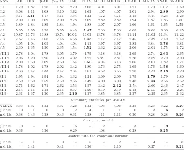
semipara-Table 3
The WMAE errors in percentage for all weeks of the Nord Pool (2003-2004) test period. Best results in each row are emphasized in bold. Like in Tables 1 and 2, measures of fit are summarized in the bottom rows.
Week AR ARX p-AR p-ARX TAR TARX MRJD MRJDX IHMAR IHMARX SNAR SNARX
II.1 1.79 1.87 1.78 1.87 2.70 3.08 3.01 3.01 1.71 1.70 1.67 1.69 II.2 3.08 3.11 3.08 3.10 3.62 3.63 4.07 4.07 3.01 2.94 2.89 2.90 II.3 3.17 3.11 3.17 3.11 3.34 3.22 4.72 4.71 3.15 3.14 3.25 3.26 II.4 2.09 2.09 2.09 2.09 2.78 3.09 2.82 2.82 1.94 1.87 1.85 1.80
II.5 1.89 1.84 1.89 1.84 1.94 1.88 2.07 2.07 1.66 1.61 1.65 1.59
V.1 5.95 5.95 5.95 5.95 5.49 5.47 7.83 7.83 6.05 6.08 6.30 6.25 V.2 10.87 10.73 10.88 10.74 10.01 10.03 13.78 13.78 11.14 11.02 11.34 11.22
V.3 7.67 7.45 7.68 7.46 5.56 5.43 7.17 7.17 7.45 7.39 7.49 7.42 V.4 4.05 4.04 4.05 4.04 4.04 4.13 3.97 3.97 3.83 3.84 3.78 3.81 V.5 2.30 2.35 2.30 2.35 1.54 1.52 2.32 2.32 2.06 2.01 1.75 1.72
VIII.1 2.78 3.04 2.78 3.05 2.79 2.79 3.18 3.18 2.69 2.74 2.63 2.65 VIII.2 2.96 3.20 2.96 3.20 3.02 3.27 2.79 2.81 2.88 2.89 2.79 2.90 VIII.3 2.09 2.50 2.09 2.50 1.64 1.56 3.04 3.13 2.06 2.01 1.82 1.71 VIII.4 1.78 2.02 1.78 2.02 2.42 2.80 2.73 2.75 1.69 1.76 1.58 1.60 VIII.5 2.33 2.47 2.33 2.47 2.34 2.61 3.52 3.55 2.28 2.29 2.18 2.20
XI.1 1.95 1.94 1.94 1.94 2.32 2.24 2.09 2.09 1.79 1.79 1.79 1.80
XI.2 2.59 2.59 2.59 2.59 2.56 2.49 3.00 3.00 2.48 2.43 2.56 2.52 XI.3 2.71 2.62 2.71 2.62 2.53 2.57 2.42 2.42 2.54 2.60 2.46 2.47 XI.4 2.14 2.16 2.13 2.16 2.37 2.29 2.59 2.59 2.13 2.11 2.24 2.24 XI.5 2.31 2.37 2.30 2.35 2.10 2.37 3.85 3.85 2.37 2.29 2.35 2.32
Summary statistics for WMAE
WMAE 3.33 3.37 3.32 3.37 3.26 3.32 4.05 4.06 3.25 3.23 3.22 3.20
# best 0 1 0 0 2 4 1 1 0 3 6 2
m.d.f.b. 0.38 0.43 0.38 0.43 0.31 0.38 1.11 1.11 0.30 0.28 0.28 0.26
Pure price models
# best 0 – 0 – 6 – 2 – 3 – 9 –
m.d.f.b. 0.36 – 0.36 – 0.29 – 1.08 0.28 – 0.25 –
Models with the exogenous variable
# best – 1 – 0 – 5 – 2 – 4 – 8
m.d.f.b. – 0.41 – 0.41 – 0.36 – 1.10 – 0.27 – 0.24
metric SNAR model (or SNARX in the class of models with temperature) is the best as far as the summary statistics are concerned. Of course, there are weeks when other models yield better forecasts. This happens mostly in May and August, when the prices are lower but more volatile. In these periods the regime switching models lead the pack. Interest-ingly, the TAR/TARX models have a relatively large number of best forecasts, but their m.d.f.b. values are (nearly) the worst, indicating that when they are wrong they miss the actual spot price by a large amount. Finally, the mean-reverting jump diffusions behave as extreme versions of the threshold models – they also have a relatively large number of best forecasts, but their m.d.f.b. values are even higher. This poor forecasting behavior may be due to the simpler autoregressive structure of the MRJD/MRDJX models. It may also be explained by the models’ similarity to Markov regime switching processes with both regimes being driven by AR(1) dynamics (with the same coefficients but different noise terms) and the switching (jump) mechanism being governed by a latent random variable. Despite the fact that Markov regime switching models fit electricity prices pretty well (Bierbrauer et al., 2007, Huisman and Mahieu, 2003), they have been reported to perform poorly in provid-ing point forecasts of hourly electricity prices (Misiorek et al., 2006) and of financial asset prices in general (Bessec and Bouabdallah, 2005).
[image:15.595.117.498.161.471.2]rows. The results closely coincide with those for the Nord Pool (1998-1999) dataset. There is no unanimous winner, but the semiparametric SNAR/SNARX models are strong leaders. Again, there are weeks when other models yield better forecasts. This happens mostly in May, when the prices drop significantly due to a warm spell, see Figure 3. Like before, in this period the TAR/TARX models lead the pack. They have a relatively large number of best forecasts and, contrary to the 1998-1999 dataset, their m.d.f.b. values are not that bad (only worse than those of the semiparametric models).
4.2. Interval forecasts
We further investigated the ability of the models to provide interval forecasts. In some applications, like risk management or bidding with a safety margin, one is more inter-ested in predicting the variability of future price movements than simply point estimates. While there is a variety of empirical studies on forecasting electricity spot prices, density or interval forecasts have not been investigated that extensively to date. More importantly, most authors looked only at their unconditional coverage (Bierbrauer et al., 2007, Misiorek et al., 2006), and some even limited the analysis to only one confidence level (Nogales and Conejo, 2006, Zhang et al., 2003). To our best knowledge, only Chan and Gray (2006) tested conditional coverage in the context of electricity spot prices. However, this was done in a Value-at-Risk setting and the focus was on one-sided prediction intervals for returns of daily aggregated electricity spot prices (point estimates and hourly prices were not considered).
For all models two sets of interval forecasts were determined: distribution-based and empirical. The method of calculating empirical prediction intervals resembles estimating Value-at-Risk via historical simulation. It is a model independent approach, which consists of computing sample quantiles of the empirical distribution of the one step ahead predic-tion errors (Weron, 2006). If the forecasts were needed for more than one step ahead then bootstrap methods could be used (for a review see Cao, 1999).
For the models driven by Gaussian noise (AR/ARX, p-AR/p-ARX, TAR/TARX, and MRJD/MRJDX) the intervals can be also computed analytically as quantiles of the Gaussian law approximating the error density (Hamilton, 1994, Ljung, 1999, Misiorek et al., 2006). The semiparametric models, on the other hand, assume a nonparametric distribution of the innovations. In their case, the ‘distribution-based’ interval forecasts can be taken as quantiles of the kernel estimator of the error density (5).
Table 4
Unconditional coverage of the 50%, 90% and 99% two-sided day-ahead prediction intervals (PI) by the actual spot price for all 12 models and the three datasets. The best results in each row are emphasized in bold, the worst are underlined.
PI AR ARX p-AR p-ARX TAR TARX MRJD MRJDX IHMAR IHMARX SNAR SNARX
California (1999-2000)
Gaussian / Kernel density intervals
50% 57.38 58.04 54.82 56.37 60.83 62.74 56.85 56.31 41.43 44.40 40.36 42.32 90% 85.95 86.07 85.60 84.88 88.57 88.75 88.33 88.04 86.13 86.07 86.37 86.19 99% 93.99 94.40 94.23 94.46 94.88 95.42 94.64 94.58 96.37 96.13 96.61 96.49
Empirical intervals
50% 39.11 40.89 39.17 41.01 50.42 54.17 43.04 42.86 36.96 39.70 36.43 37.56
90% 84.94 84.35 85.24 84.46 87.50 88.15 87.92 87.32 85.36 85.18 85.54 85.36 99% 95.83 95.65 96.43 96.13 96.13 96.19 96.43 96.49 95.89 95.71 96.19 95.95
Nord Pool (1998-1999)
Gaussian / Kernel density intervals
50% 82.65 80.30 81.52 79.02 90.80 90.48 86.19 85.77 58.87 53.33 61.67 56.93 90% 98.63 98.57 98.48 98.42 99.70 99.79 98.57 98.60 97.26 97.17 97.11 96.99
99% 99.94 99.94 99.88 99.88 100.00 100.00 99.91 99.91 100.00 100.00 100.00 100.00
Empirical intervals
50% 55.54 48.63 55.36 48.51 76.73 75.89 61.10 59.67 54.49 49.29 54.08 51.46
90% 97.17 96.64 97.17 96.64 99.08 99.20 97.23 97.17 96.99 96.90 96.88 96.79 99% 100.00 100.00 100.00 100.00 100.00 100.00 100.00 100.00 100.00 100.00 100.00 100.00
Nord Pool (2003-2004)
Gaussian / Kernel density intervals
50% 80.63 80.42 80.71 80.42 89.38 88.66 80.30 80.30 61.25 61.10 61.79 62.05 90% 96.43 96.40 96.43 96.37 97.44 97.56 95.95 95.95 94.82 94.85 94.49 94.40
99% 97.89 97.95 97.89 97.95 99.08 99.08 97.80 97.80 98.57 98.66 98.60 98.57
Empirical intervals
50% 57.08 55.68 57.14 55.80 77.50 77.29 61.99 61.40 57.41 57.47 58.21 58.15 90% 94.26 94.35 94.26 94.32 96.01 96.25 94.61 94.61 94.49 94.52 94.23 94.23
99% 98.48 98.45 98.48 98.48 99.35 99.43 98.78 98.78 98.48 98.39 98.45 98.42
itself and resembles it much more than any parametric distribution. Third, models with and without the exogenous variable (within the same class, e.g. AR and ARX) yield similar PI. Fourth, the results for both Nord Pool test samples are similar, despite the fact that the price behavior was different. At the same time they are different from the results for the California sample. For California, the threshold models exhibit a very good performance – their empirical, as well as, 90% Gaussian intervals have the best or nearly the best coverage. The semiparametric models are next in line, failing mainly in the 50% empirical PI category. The simple linear models are overall the worst. For the Nord Pool test samples the situation is different. Here the semiparametric models provide the best or nearly the best PI, while the TAR/TARX models are the worst (except for the 99% intervals in 2004). Finally, the mean-reverting jump diffusions yield relatively good (unconditional) coverage of the 99% PI and their results resemble those of the threshold models much more than those of the simple linear models. The latter fact can be attributed to the similar, non-linear structure of both models.
asymp-totically asχ2(1) and the latter asχ2(2). Moreover, if we condition on the first observation,
then the conditional coverage LR test statistics is the sum of the other two.
The conditional coverage LR statistics for the ‘X’ models are plotted in Figures 4-6 (mod-els without the exogenous variable yield similar PI and, hence, similar LR statistics). They were computed for the 24 hourly time series separately. It would not make sense to compute the statistics jointly for all hours, since, by construction, the forecasts for consecutive hours are correlated – predictions for all 24 hours of the next day are made at the same time using the same information set.
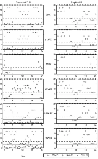
None of the tested models is perfect. There are always hours during which the uncon-ditional coverage is poor and/or the independence of predictions for consecutive days is violated leading to high values of the conditional coverage LR statistics. For the California dataset this happens mainly during late night and early morning hours, see Figure 4. Taking a global look at all hours, we can observe that the semiparametric models yield the best conditional coverage (with the kernel density PI being slightly better than the empirical ones). The TARX specification performs particularly bad in terms of its 50% Gaussian PI; on the other hand, its empirical PI have a better coverage than all models except IHMARX and SNARX. The MRJDX model behaves comparably to the simple linear models, except for a slightly better coverage of the Gaussian PI.
For the Nord Pool (1998-1999) dataset only the kernel density PI of the semiparametric models yield acceptable conditional coverage, though, most of the test statistics for the 99% PI exceed the 1% significance level, see Figure 5. All empirical and nearly all Gaussian intervals (except the 90% PI for ARX and p-ARX models) fail the LR test miserably. The worst performing model is TARX, which is in line with the results presented in Table 4. Note, that many of the test values (especially for the 99% and 90% PI) could not be computed due to lack of observations exceeding the corresponding PI, these values were set to 20 to allow visualization in the figures.
Test results for the Nord Pool (2003-2004) dataset resemble more those of the California sample – the PI exhibit a significantly better coverage than in 1999, see Figure 6. This time the troublesome hours are the morning ones (in terms of independence) and mid-day and evening hours (in terms of unconditional coverage). Like for the two other datasets, the semiparametric models have the lowest test statistics. Only this time the empirical PI yield better conditional coverage than the kernel density intervals. The better performance of the empirical PI is even more visible for the Gaussian models. This extremely good coverage is in sharp contrast to the results for the Nord Pool (1998-1999) dataset.
5. Conclusions
1 6 12 18 24 0 5 10 15 20 Gaussian/KD PI ARX
1 6 12 18 24
0 5 10 15 20 Empirical PI
1 6 12 18 24
0 5 10 15 20 p−ARX
1 6 12 18 24
0 5 10 15 20
1 6 12 18 24
0 5 10 15 20 TARX
1 6 12 18 24
0 5 10 15 20
1 6 12 18 24
0 5 10 15 20 MRJDX
1 6 12 18 24
0 5 10 15 20
1 6 12 18 24
0 5 10 15 20 IHMARX
1 6 12 18 24
0 5 10 15 20
1 6 12 18 24
0 5 10 15 20 SNARX Hour
1 6 12 18 24
[image:19.595.145.468.136.650.2]0 5 10 15 20 Hour 50% PI 90% PI 99% PI
1 6 12 18 24 0 5 10 15 20 Gaussian/KD PI ARX
1 6 12 18 24
0 5 10 15 20 Empirical PI
1 6 12 18 24
0 5 10 15 20 p−ARX
1 6 12 18 24
0 5 10 15 20
1 6 12 18 24
0 5 10 15 20 TARX
1 6 12 18 24
0 5 10 15 20
1 6 12 18 24
0 5 10 15 20 MRJDX
1 6 12 18 24
0 5 10 15 20
1 6 12 18 24
0 5 10 15 20 IHMARX
1 6 12 18 24
0 5 10 15 20
1 6 12 18 24
0 5 10 15 20 SNARX Hour
1 6 12 18 24
[image:20.595.145.469.133.656.2]0 5 10 15 20 Hour 50% PI 90% PI 99% PI
1 6 12 18 24 0 5 10 15 20 Gaussian/KD PI ARX
1 6 12 18 24
0 5 10 15 20 Empirical PI
1 6 12 18 24
0 5 10 15 20 p−ARX
1 6 12 18 24
0 5 10 15 20
1 6 12 18 24
0 5 10 15 20 TARX
1 6 12 18 24
0 5 10 15 20
1 6 12 18 24
0 5 10 15 20 MRJDX
1 6 12 18 24
0 5 10 15 20
1 6 12 18 24
0 5 10 15 20 IHMARX
1 6 12 18 24
0 5 10 15 20
1 6 12 18 24
0 5 10 15 20 SNARX Hour
1 6 12 18 24
[image:21.595.146.467.132.651.2]0 5 10 15 20 Hour 50% PI 90% PI 99% PI
Furthermore, taking into account all datasets, we can conclude that the semiparametric models (IHMAR/IHMARX and SNAR/SNARX) usually lead to better point forecasts than their Gaussian competitors. More importantly, they have the potential to perform well un-der different market conditions, unlike the spike-preprocessed linear models or the threshold regime switching specifications. Only for the California test period and only in the calm weeks the SNAR/SNARX models are dominated by the p-AR/p-ARX models. Their per-formance is much better for the Nord Pool datasets, they are the best in terms of all three summary statistics. The IHMAR/IHMARX models follow closely.
Regarding interval forecasts, the two semiparametric model classes are better (on aver-age) than the other models both in terms of unconditional and conditional coverage. In particular, only the kernel density PI of the semiparametric models yield acceptable values of Christoffersen’s test statistics for all hours and all three datasets. The Nord Pool (1998-1999) sample is particularly discriminatory in this respect and shows that empirical PI may be very misleading.
There is no clear outperformance of one semiparametric model by the other in terms of interval forecasts. Yet, the slightly better point predictions of the smoothed nonparametric approach allow us to conclude that the SNAR/SNARX models are an interesting tool for short-term forecasting of hourly electricity prices.
Acknowledgements
The authors would like to thank James Taylor and two anonymous referees for insightful and detailed comments and suggestions. Thanks are due also to the participants of seminars at Humboldt-Universit¨at zu Berlin, University of Z¨urich, Wroc law University of Economics, and conference participants of FindEcon’2007, AMaMeF’2007, Energy Risk’2007 and IGSSE 2007 Workshop on Energy. The meteorological data were kindly provided by the Swedish Meteorological and Hydrological Institute.
References
Ball, C.A., and W.N. Torous (1983). A simplified jump process for common stock returns,Journal of Finance and Quantitative Analysis18(1), 53-65.
Bessec, M., and O. Bouabdallah (2005). What causes the forecasting failure of Markov-switching models? A Monte Carlo study,Studies in Nonlinear Dynamics and Econometrics9(2), Article 6.
Bierbrauer, M., C. Menn, S.T. Rachev, and S. Tr¨uck (2007). Spot and derivative pricing in the EEX power market,Journal of Banking & Finance31, 3462-3485.
Bunn, D.W. (2000). Forecasting loads and prices in competitive power markets,Proc. IEEE 88(2), 163-169. Cao, R. (1999). An overview of bootstrap methods for estimating and predicting time series, Test 8(1),
95-116.
Cao, R., A. Cuevas, and W. Gonz´alez-Manteiga (1993). A comparative study of several smoothing methods in density estimation.Computational Statistics & Data Analysis17, 153-176.
Cao, R., J.D. Hart, and A. Saavedra (2003). Nonparametric maximum likelihood estimators for AR and MA time series,Journal of Statistical Computation and Simulation73(5), 347-360.
Chan, K.F., and P. Gray (2006). Using extreme value theory to measure value-at-risk for daily electricity spot prices,International Journal of Forecasting22, 283-300.
Chan, K.F., P. Gray, and B. van Campen (2008). A new approach to characterizing and forecasting electricity price volatility,International Journal of Forecasting, forthcoming.
Christoffersen, P. (1998). Evaluating interval forecasts,International Economic Review 39(4), 841-862. Conejo, A.J., J. Contreras, R. Esp´ınola, and M.A. Plazas (2005). Forecasting electricity prices for a
Cont, R., and P. Tankov (2003). Financial Modelling with Jump Processes, Chapman & Hall / CRC Press. Contreras, J., R. Esp´ınola, F.J. Nogales, and A.J. Conejo (2003). ARIMA models to predict next-day
electricity prices,IEEE Trans. Power Systems 18(3), 1014-1020.
Cuaresma, J.C., J. Hlouskova, S. Kossmeier, and M. Obersteiner (2004). Forecasting electricity spot prices using linear univariate time-series models,Applied Energy77, 87-106.
Garcia, R.C., J. Contreras, M. van Akkeren, and J.B.C. Garcia (2005). A GARCH forecasting model to predict day-ahead electricity prices,IEEE Transactions on Power Systems20(2), 867-874.
Hamilton, J. (1994). Time Series Analysis, Princeton University Press.
H¨ardle, W., H. L¨utkepohl, and R. Chen (1997). A review of nonparametric time series analysis,International Statistical Review 65, 49-72.
H¨ardle, W., M. M¨uller, S. Sperlich, and A. Werwatz (2004). Nonparametric and Semiparametric Models, Springer, Heidelberg.
Hsieh, D.A., and C.F. Manski (1987) Monte Carlo evidence on adaptive maximum likelihood estimation of a regression,Annals of Statistics 15, 541-551.
Huisman, R., and R. Mahieu (2003). Regime jumps in electricity prices,Energy Economics25, 425-434. Johnson, B., and G. Barz (1999). Selecting stochastic processes for modelling electricity prices. In: Energy
Modelling and the Management of Uncertainty, Risk Books, London.
Jones, M.C., J.S. Marron, and S.J. Sheather (1996). A brief survey of bandwidth selection for density estimation.Journal of the American Statistical Association91, 401-407.
Kaminski, V. (1997). The challenge of pricing and risk managing electricity derivatives. In: The US Power Market, Risk Books, London.
Karakatsani, N., and D. Bunn (2008). Forecasting electricity prices: The impact of fundamentals and time-varying coefficients,International Journal of Forecasting, forthcoming.
Kirschen, D.S., and G. Strbac (2004). Fundamentals of Power System Economics. John Wiley & Sons, Chichester.
Knittel, C.R., and M.R. Roberts (2005). An empirical examination of restructured electricity prices,Energy Economics27(5), 791-817.
Kreiss, J-P. (1987). On adaptive estimation in stationary ARMA processes,Annals of Statistics15, 112-133. Ljung, L. (1999). System Identification – Theory for the User, 2nd ed., Prentice Hall, Upper Saddle River. Misiorek, A., S. Tr¨uck, and R. Weron (2006). Point and Interval Forecasting of Spot Electricity Prices: Linear vs. Non-Linear Time Series Models,Studies in Nonlinear Dynamics & Econometrics10(3), Article 2. Nogales, F., and A. Conejo (2006). Electricity price forecasting through transfer function models,Journal
of the Operational Research Society57, 350-356.
Panagiotelis, A., and M. Smith (2008). Bayesian forecasting of intraday electricity prices using multivariate skew-elliptical distributions,International Journal of Forecasting, forthcoming.
Shahidehpour, M., H. Yamin, and Z. Li (2002). Market Operations in Electric Power Systems: Forecasting, Scheduling, and Risk Management, Wiley.
Silverman, B.W. (1986). Density Estimation for Statistics and Data Analysis, Chapman & Hall, London. Tong, H., and K.S. Lim (1980). Threshold autoregression, limit cycles and cyclical data, Journal of the Royal
Statistical Society B 42, 245-292.
Weron, R. (2006). Modeling and forecasting electricity loads and prices: A statistical approach, Wiley, Chichester.
Weron, R. (2008). Market price of risk implied by Asian-style electricity options and futures. Energy Economics30, 1098-1115.
Weron, R. (2008). Forecasting wholesale electricity prices: A review of time series models. In: Financial Markets: Principles of Modelling, Forecasting and Decision-Making, W. Milo, P. Wdowi´nski (eds.), FindEcon Monograph Series, WU L, L´od´z.
Zhang, L., P.B. Luh, and K. Kasiviswanathan (2003). Energy clearing price prediction and confidence interval estimation with cascaded neural networks,IEEE Trans. Power Systems 18, 99-105.