http://dx.doi.org/10.4236/ajor.2016.61010
How to cite this paper: Quaddoura, R. (2016) An O(n) Time Algorithm for Scheduling UET-UCT of Bipartite Digraphs of
An
O
(
n
) Time Algorithm for Scheduling
UET-UCT of Bipartite Digraphs of Depth
One on Two Processors
Ruzayn Quaddoura
Department of Computer Science, Faculty of Information Technology, Zarqa University, Zarqa, Jordan
Received 17 November 2015; accepted 24 January 2016; published 28 Janaury 2016
Copyright © 2016 by author and Scientific Research Publishing Inc.
This work is licensed under the Creative Commons Attribution International License (CC BY). http://creativecommons.org/licenses/by/4.0/
Abstract
Given n unit execution time (UET) tasks whose precedence constraints form a directed acyclic graph, the arcs are associated with unit communication time (UCT) delays. The problem is to schedule the tasks on two identical processors in order to minimize the makespan. Several poly-nomial algorithms in the literature are proposed for special classes of digraphs, but the complexi-ty of solving this problem in general case is still a challenging open question. We present in this paper an O(n) time algorithm to compute an optimal schedule for the class of bipartite digraphs of depth one.
Keywords
Scheduling, Makespan, Precedence Constraints, Bipartite Graph, Optimal Algorithm
1. Introduction
The problem of scheduling a set of tasks on a set of identical processors under a precedence relation has been studied for a long time. A general description of the problem is the following. There are n tasks that have to be executed by m identical processors subject to precedence constraints and (may be without) communication de-lays. The objective is to schedule all the tasks on the processors such that the makespan is the minimum. Gener-ally, this problem can be represented by a directed acyclic graph G=
(
V E,)
called a task graph. The set of vertices V corresponds to the set of tasks and the set of edges E corresponds to the set of precedence constrains. With every vertex i, a weight pi is associated that represents the execution time of the task i, and with every edge( )
i j, , a weight cij is associated that represents the communication time between the tasks i and j. If( )
i j, ∈Eand the task i starts its execution at time t on a processor P, then either j starts its execution on P at time greater than or equal to t+ pj, or j starts its execution on some other processor at time greater than or equal to
According to the three field notation scheme introduced in [1] and extended in [2] for scheduling problems with communication delays, this problem is denoted as Pm|prec p c, i, ij|Cmax.
A large amount of work in the literature studies this problem with a restriction on its structure: the time of execution of every task is one unit execution time (UET), the number of processors m is fixed, the communica-tion delays are neglected, constant or one unit (UCT), or special classes of task graph are considered. We find In this context, the problem P2|prec p, i =1 |Cmax, is polynomial [3] [4], i.e. when the communication delays are not taken into account. On the contrary, the problem P3|prec p, i=1 |Cmax remains an open question [5].
The problem of two processors scheduling with communication delays is extensively studied [6] [7]. In par-ticular, it is proven in [8] that the problem P2|prec=binary tree,pi=1,cij =c C| max is NP-hard where c is a large integer, whereas this problem is polynomial when the task graph is a complete binary tree.
A challenging open problem is the two processors scheduling with UET-UCT, i.e. the problem
2| , i 1, ij 1 | max
P prec p = c = C for which the complexity is unknown. However, several polynomial algorithms have been shown for special classes of task graphs, especially for trees [9] [10], interval orders [11] and a sub- class of series parallel digraphs [12]. In this paper we present an O n
( )
time algorithm to compute an optimal algorithm for the class of bipartite digraphs of depth one, that is the digraphs for which every vertex is either a source (without predecessors) or a sink (without successors).2. Scheduling UET-UCT for a Bipartite Digraph of Depth One on Two Processors
2.1. Preliminaries
A schedule UET-UCT on two processors for a general directed acyclic digraph G=
(
V E,)
is defined by a functionσ
:V →+×{
P P1, 2}
,σ
( ) (
v = t Pv, i)
,i=1, 2 where tv is the time for which the task v is executedand Pi the processor on which the task v is scheduled. A schedule
σ
is feasible if: a) ∀u v, ∈V, ifu
≠
v
thenσ
( )
u ≠σ
( )
vb) If
( )
u v, ∈E then tu+ ≤1 tv if u and v are scheduled on the same processor, and tu+ ≤2 tv if u and vare scheduled on distinct processors.
A time t of a schedule
σ
is said to be idle if one of the processors is idle during this time. The makespanmax
C or the length of a schedule
σ
is the last non-idle time ofσ
, that is:( ) ( )
{
}
max max : , i , 1 or 2
C = t ∃ ∈v V
σ
v = t P i=A schedule
σ
is optimal if Cmax is the minimum among all feasible schedules.Let G=
(
BW E,)
be a bipartite digraph of depth one. Since every vertex of G is either a source or a sink, there exists always a feasible schedule such that the sources B are executed before executing the sinks W. Our algorithm for solving the problem under consideration produces an optimal schedule satisfies this condition and that we called a natural schedule defined as follows.Definition 1 Let G=
(
BW E,)
be a bipartite digraph of depth one. A natural schedule of G is obtained by scheduling first the sources B then the sinks W starting from the processor P1 and alternating between P1 and P2 such that the resulting schedule is optimal.The definition of a natural schedule
σ
of a bipartite digraph of depth one G=(
BW E,)
implies the fol-lowing properties:1) The number of sources executed on P1 is B 2 and the number of sources executed on P2 is 2
B .
2) If B is even then:
a)
σ
contains at most 2 idle times, the first is at time B 2 1+ , and the second is at time Cmax. b) If B 2 1+ is an idle time then P2 is idle at this time (may be P1 also).3) If B is odd then:
a)
σ
contains at most 3 idle times, the first is at time B 2, the second is at time B 2 + 1, and the third is at time Cmax.b) If B 2 or B 2 + 1 is an idle time then P2 is idle at this time and P1 is non. 4) B W 2 ≤Cmax ≤ B W 2 + 1.
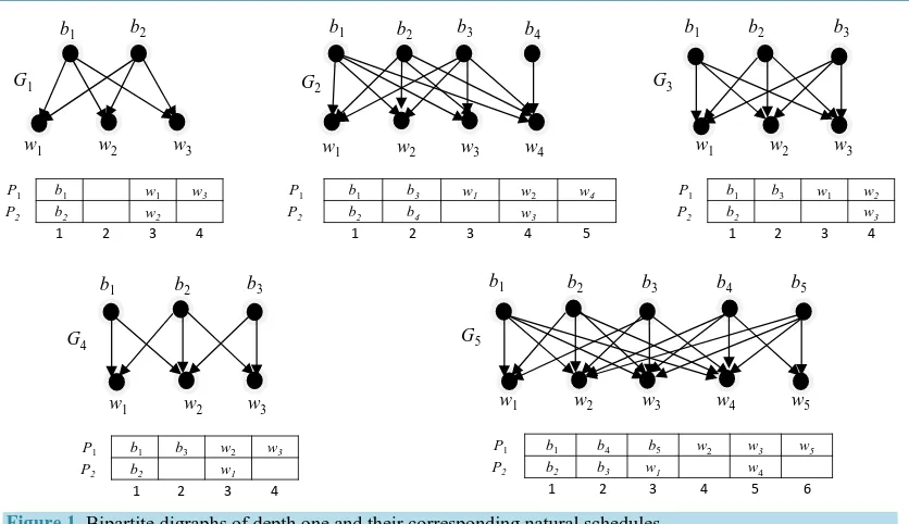
Figure 1. Bipartite digraphs of depth one and their corresponding natural schedules.
max 2 1
C = BW + . Figure 1 illustrates some bipartite digraphs of depth one and their corresponding natu-ral schedules.
2.2. Scheduling Algorithm
The idea of solving the problem P2|prec=bipartite of depth one p , j =1,cij =1 |Cmax is to determine the ne-cessary and sufficient conditions to exist idle times in a natural schedule of the task graph. In the following, we consider G=
(
BW E,)
is a bipartite digraph of depth one where B is the set of sources and W is the set of sinks, andσ
is a natural schedule for G. A vertex b∈B (w W∈ ) is called universal if d b( )
=W( )
(
d w = B)
. We distinguish two cases, B is even and B is odd.Lemma 2Assume that B is even.
1) The two processors P1 and P2 are idle at time B 2 1+ if and only if G is a bipartite complete. 2) The processor P2 only is idle at time B 2 1+ if and only if one of the following holds:
a) Every vertex of B is universal except exactly one. b) Every vertex of W is universal except exactly one.
Proof. 1) If G is a bipartite complete then obviously P1 and P2 must be idle at time B 2 1+ . The inverse, let b and w be a source and a sink of G. If b is not adjacent to w, then we can schedule b on P2 at time B 2 and w on P1 at time B 2 1+ , a contradiction. So b must be adjacent to w, therefore G is a bipartite complete.
2) Assume that P2 only is idle at time B 2 1+ and the conditions a and b are not hold. Then, there exist
1, 2
b b ∈B and w w1, 2∈W such that b b w1, 2, 1 and w2 are all not universal. If
{
b b w w1, 2, 1, 2}
is a stable set, i.e. no two vertices are adjacent, we can schedule b b1, 2 on P P1, 2 at time B 2 and w w1, 2 on P P1, 2 at time B 2 1+ , a contradiction. If{
b b w w1, 2, 1, 2}
is not a stable set then we can suppose that b w1 1∈E. Since1
b and w1 are not universal, there exist w W∈ and b∈B such that b w1 ∉E and bw1∉E. But now, we can schedule b1,b on P P1, 2 respectively at time B 2, and w1, w on P P1, 2 respectively at time B 2 1+ , a contradiction.
The inverse, suppose that every vertex of B is universal except exactly one. Since B is even, there exist
1, 2
b b ∈B scheduled on P P1, 2 at time B 2. By 1, the two processors can’t be idle at time B 2 1+ . If P2
is not idle at time B 2 1+ , then both b1 and b2 are not universal, a contradiction. In a similar way we prove the case b.
Notice that if B (or W) contains exactly one non-universal vertex b then the vertex of W which is independent of b is also non-universal but it is not necessary unique (seeFigure 1). Algorithm Schedule_|B|_is_even (G) constructs a natural schedule for G=
(
BW E,)
if B is even, Lemma 2 proves its correctness.b1 b2
G1
w1 w2 w3
b1 b2
G2
w1 w2 w3 w4
b3 b4 b1 b2
G3
w1 w2 w3
b3
b1 b2
G4
w1 w2 w3
b3 b1 b2
G5
w1 w2 w3 w4
b3 b4 b5
w5
P1 b1 w1 w3
P2 b2 w2
1 2 3 4
P1 b1 b3 w2 w3
P2 b2 w1
1 2 3 4
P1 b1 b3 w1 w2
P2 b2 w3
1 2 3 4
P1 b1 b4 b5 w2 w3 w5
P2 b2 b3 w1 w4
1 2 3 4 5 6
P1 b1 b3 w1 w2 w4
P2 b2 b4 w3
Algorithm Schedule_|B|_is_even (G)
( )
{
}
1 :
B = ∈b B d b =W
( )
{
}
2 :
B = b∈B d b <W
( )
{
}
1 :
W = w W d w∈ = B
( )
{
}
2 :
W = w W d w∈ < B
If B1 = B and W1 =W then
Schedule B1 alternately on P1 and P2 at times 1, 2,,B 2
Schedule W1 alternately on P1 and P2 at times B 2 1,+ ,BW 2 + 1 Else if B2 =1 or W2 =1 then
Let b∈B2 and w W∈ 2 such that bw∉E
Schedule b on P2 at time B 2 and w on P1 at time B 2 1+
Schedule B−
{ }
b alternately on P1 and P2 at times 1, 2,,B 2Schedule W−
{ }
w alternately on P1 and P2 at times B 2 1,+ ,BW 2 + 1 Else let b b1, 2∈B2 and w w1, 2∈W2 such that b w1 1∉E b w, 2 2∉ESchedule b1 on P1 and b2 on P2 at time B 2 Schedule w2 on P1 and w1 on P2 at time B 2 1+
Schedule B−
{
b b1, 2}
alternately on P1 and P2 at times 1, 2,,B 2 1−Schedule W−
{
w w1, 2}
alternately on P1 and P2 at times B 2+2,,BW 2Figure 1 shows the construction of natural schedules of the graphs G1 and G2 resulting from the algo-rithm Schedule_|B|_is_even (G).
Lemma 3 Assume that B is odd.
1) The processor P2 is idle at times B 2 and B 2 + 1 if and only if G is a bipartite complete. 2) The processor P2 is idle at time B 2 and not idle at time B 2 + 1 if and only if
a) There is w W∈ such that d w
( )
= B −1 b) For every w W∈ , d w( )
= B or B −1.3) The processor P2 is idle at time B 2 + 1 and not idle at time B 2 if and only if a) There is w W∈ such that d w
( )
≤ B −2b) For every w W∈ for which d w
( )
≤ B −2 and for every b∈N w( )
, d b( )
=W −1 where N w( )
is the set of non-neighbors of w.Proof. 1) If G is a bipartite complete then obviously P2 is idle at times B 2 and B 2 + 1. The in-verse, let b and w be a source and a sink of G. If b is not adjacent to w, then we can schedule b on P1 at time
2
B
and w on P2 at time B 2 or at time B 2 + 1 according to the adjacency relation between the source scheduled on P1 at time B 2 −1 and w, a contradiction. So b must be adjacent to w, therefore G is a bipartite complete.
2) Assume that P2 is idle at time B 2 and not idle at time B 2 + 1. The vertex w W∈ scheduled
onP2 at time B 2 + 1 is of degree less than or equal to B −1, since it must be independent of the vertex b∈B scheduled on P1 at time B 2. If there is a vertex w W∈ such that d w
( )
≤ B −2, then we can schedule w on P2 at time B 2 and two vertices from B independent of w on P1 at times B 2 − 1 and2
B
, a contradiction.
The inverse, by 1, the processor P2 is not idle at time B 2 or at time B 2 + 1. If P2 is not idle at time B 2 then the vertex scheduled at this time would be of degree less than or equal to B−2, a contra-diction.
3) Assume that P2 is idle at time B 2 + 1 and not idle at time B 2. The vertex w W∈ scheduled on P2 at time B 2 is of degree less than or equal to B−2, since it must be independent of the two ver-tices b b1, 2∈B scheduled on P1 at times B 2 −1 and B 2. Let w W∈ such that d w
( )
≤ B −2and let b∈N w
( )
such that d b( )
≤W −2. Now, we can schedule 𝑤𝑤 on P2 at time B 2, b and another vertex b′ independent of w on P1 at time B 2 and B 2 − 1 respectively, and schedule a vertex w′ independent of b on P2 at time B 2 + 1, a contradiction. The inverse, by 1 and 2, the processor P2 can’t be idle at time B 2 and any vertex scheduled on P2 at time B 2 must be of degree less than or equal to B −2. The processor P2 is idle at time B 2 +1, otherwise the vertex scheduled on P1 at time2
B
is of degree less than or equal to W −2, a contradiction.
To construct a natural schedule for G when B is odd, we need to the Procedure Two_Vertices (G). This procedure return 1 if the condition 3.b of Lemma 3 holds, and return two vertices w, b such that d w
( )
≤ B−2,( )
Procedure Two_Vertices (G)
( )
{
}
{
3}
3 : 2 1, , W
W = w W d w∈ ≤ B − = w w For i=1 to W3
( )
{
1, 2, ,}
i i i
i k
N w = b b b
For j=1 to k If
( )
i 2j
d b ≤W − then Return
(
, i)
i jw b
Return 1.
Algorithm Schedule_|B|_is_odd (G) constructs a natural schedule for G=
(
BW E,)
if B is odd. Lemma 3 proves its correctness.Algorithm Schedule_|B|_is_odd (G)
( )
{
}
1 :
B = ∈b B d b =W
( )
{
}
2 :
B = b∈B d b <W
( )
{
}
1 :
W = w W d w∈ = B
( )
{
}
2 : 1
W = w W d w∈ = B −
( )
{
}
3 : 2
W = w W d w∈ ≤ B −
If B1 = B and W1 =W then
Schedule a vertex b∈B on P1 at time B 2 Schedule a vertex w W∈ on P1 at time B 2 + 1
Schedule B−
{ }
b alternately on P1 and P2 at times 1,,B 2 − 1Schedule W−
{ }
w alternately on P1 and P2 at times B 2 + 2,,BW 2 + 1 Else if W3 =0 thenLet w W∈ 2 and b∈B2 such that bw∉E Schedule b on P1 at time B 2
Schedule w on P2 at time B 2 + 1
Schedule B−
{ }
b alternately on P1 and P2 at times 1,,B 2 − 1Schedule W−
{ }
w alternately on P1 and P2 at times B 2 + 1,,BW 2 + 1 Else If Two_Vertices (G) = 1 thenLet w W∈ 3 and b b1, 2∈B2 such that b w b w1 , 2 ∉E
Schedule b b1, 2 on P1 at times B 2 − 1 and B 2 Schedule w on P2 at time B 2
Schedule B−
{
b b1, 2}
alternately on P1 and P2 at times 1,,B 2 − 1 Schedule a vertex w′ ∈W−{ }
w on P1 at time B 2 + 1Schedule W−
{
w w, ′}
alternately on P1 and P2 at times B 2 +2,,BW 2 + 1 Else let(
w b,)
= Two_Vertices (G)Let b1∈B2−
{ }
b and w1∈W2W3−{ }
w such that b w bw1 , 1∉ESchedule b b1, on P1 at times B 2 − 1 and B 2 respectively Schedule w w, 1 on P2 at times B 2 and B 2 + 1 respectively Schedule B−
{
b b1,}
alternately on P1 and P2 at times 1,,B 2 − 1Schedule W−
{
w w, 1}
alternately on P1 and P2 at times B 2 +1,,BW 2Figure 1shows the construction of natural schedules of the graphs G G3, 4 and G5 resulting from the algo-rithm Schedule_|B|_is_odd (G).
2.3. Complexity
We assume that G=
(
BW E,)
is represented by its adjacency lists, so the set of neighbors and the set of non neighbors of every vertex of G are known already. In this supposition, we can check easily that any step (except the step Two_Vertices (G)) of the two algorithms Schedule_|B|_is_even (G) and Schedule_|B|_is_ odd (G) can be executed either within a constant time or within an O n( )
time where BW =n. Let’s prove that the Procedure Two_Vertices (G) runs within O B( )
time.The worst case of this Procedure occurs when its result is 1. In this case, for any w w1, 2∈W3,
( )
1( )
2N w N w = ∅, otherwise, a vertex b independent of w1 and w2 would be of degree less than or equal to W −2 . So the number of comparisons of if statement in this procedure is equal to at most
( )
( )
3
1 W
time of our scheduling algorithm is O n
( )
.3. Conclusion
We have presented an O n
( )
time algorithm for the optimal schedule of bipartite digraphs of depth one with UET-UCT on two processors. The complexity of this problem for general directed acyclic graphs is still an open question. We believe that our algorithm can be used to solve this problem in general as follow: Consider a topo-logical sort of a directed acyclic graph G. The linear ordering defined by this topological sort decomposes G into consecutives bipartite digraphs of depth one. The schedule obtained by the concatenation of the schedules of these bipartite digraphs is a feasible schedule or may be modified to a feasible schedule of G. Now, if we can determine the necessary and sufficient conditions to exist idle times in this feasible schedule then we can deter-mine the complexity of this problem. This is a useful guide and foundation for future research.Acknowledgements
This research is funded by the Deanship of Research and Graduate Studies in Zarqa University/Jordan. The au-thor is grateful to anonymous referee’s suggestion and improvement of the presentation of this paper.
References
[1] Graham, R.L., Lawler, E.L., Lenstra, J.K. and Rinnooy Kan, A.H.G. (1979) Optimization and Approximation in De-terministic Scheduling: A Survey. Annals of Discrete Mathematics, 5, 287-326.
http://dx.doi.org/10.1016/S0167-5060(08)70356-X
[2] Veltman, B., Lageweg, B.J. and Lenstra, L.K. (1990) Multiprocessor Scheduling with Communication Delays. Parallel Computing, 16, 173-182. http://dx.doi.org/10.1016/0167-8191(90)90056-F
[3] Coffman Jr., E.G. and Graham, R.L. (1972) Optimal Scheduling for Two-Processor Systems. Acta Informatica, 1, 200- 213. http://dx.doi.org/10.1007/BF00288685
[4] Fujii, M., Kasami, T. and Ninomiya, K. (1969) Optimal Sequencing of Two Equivalent Processors. SIAM Journal on Applied Mathematics, 17, 784-789. http://dx.doi.org/10.1137/0117070
[5] Garey, M.R. and Johnson, D.S. (1979) Computers and Intractability: A Guide to the Theory of NP-Completeness. Freeman.
[6] Chrétienne, P. and Picouleau, C. (1995) Scheduling with Communication Delays: A Survey. In: Scheduling Theory and Its Applications, John Wiley & Sons.
[7] Norman, M.G., Pelagatti, S. and Thanisch, P. (1995) On the Complexity of Scheduling with Communication Delay and Contention. Parallel Processing Letters, 5, 331-341. http://dx.doi.org/10.1142/S012962649500031X
[8] Afrati, F., Bampis, E., Finta, L. and Mili, I. (2005) Scheduling Trees with Large Communication Delays on Two Iden-tical Processors. Journal of Scheduling, 8, 179-190. http://dx.doi.org/10.1007/s10951-005-6366-3
[9] Varvarigou, T., Roychowdhury, V.P., Kailath, T. and Lawler, E. (1996) Scheduling in and out Forests in the Presence of Communication Delays. IEEE Transactions on Parallel and Distributed Systems, 7, 1065-1074.
http://dx.doi.org/10.1109/71.539738
[10] Veldhorst, M. (1993) A Linear Time Algorithm to Schedule Trees with Communication Delays Optimally on Two Machines. Technical Report COSOR 93-07, Department of Math, and Computer Science, Eindhoven University of Technology, Eindhoven.
[11] Ali, H. and El-Rewini, H. (1993) The Time Complexity of Scheduling Interval Orders with Communication Is Poly-nomial. Parallel Processing Letters, 3, 53-58. http://dx.doi.org/10.1142/S0129626493000083