Glass Ceiling or Sticky Floor? Examining the Gender Pay Gap across the Wage Distribution in Urban China, 1987 2004

(1)

Munich Personal RePEc Archive

Glass Ceiling or Sticky Floor? Examining

the Gender Pay Gap across the Wage

Distribution in Urban China, 1987-2004

Chi, Wei and Li, Bo

May 2007

Online at

https://mpra.ub.uni-muenchen.de/3544/

(2)

Glass Ceiling or Sticky Floor? Examining the Gender Pay Gap

across the Wage Distribution in Urban China, 1987-2004

Wei Chi

School of Economics and Management Tsinghua University, China

chiw@sem.tsinghua.edu.cn

Bo Li

School of Economics and Management Tsinghua University, China

libo@sem.tsinghua.edu.cn

(3)

2

Glass Ceiling or Sticky Floor? Examining the Gender Pay Gap across the Wage Distribution in Urban China, 1987-2004

Abstract:

Using 1987, 1996, and 2004 data, we show that the gender pay gap in the Chinese urban labor market has increased across the wage distribution, and the increase was greater at the lower quantiles. We interpret this as evidence of the “sticky floor” effect. We use the reweighting and recentered influence function projection method proposed by Firpo, Fortin, Lemieux (2005) to decompose gender pay differentials across the wage distribution. We find that the gender differences in the return to labor market characteristics, also known as the “discrimination effect” or “unexplained gender pay gap”, contribute most to the increase in the overall gender pay gap. The Firpo, Fortin, and Lemieux method allows us to further decompose the gender pay gap into the contribution of each individual variable. We find that the “sticky floor” effect may be associated with a particularly low paid group of female production workers with relatively less education working in non-state owned enterprises.

JEL code: J3

(4)

3

1. Introduction

Recent decades have witnessed a significant increase in the gender pay inequality

in China.1 According to the National Bureau of Statistics of China (NBSC), the ratio

of female to male employees’ average earnings had fallen by eight percentage points

from 1987 to 2004. This is despite the fact that female employees’ education

attainment had risen faster than male employees. The percentage of female workers

who received education at the college level or higher had increased by five folds from

1987 to 2004, while that for male workers had only nearly tripled.

Two reasons may contribute to the explanation of the rising gender pay gap in a

transitional country such as China. Firstly, during the transition to a market economy,

the return to workers’ productivity characteristics such as education attainment and

employment experiences tends to increase; if men and women have different

characteristics, the gender pay gap may rise as the result of the increasing return to

these characteristics. Secondly, the rising gender pay gap could also be the result of

escalating discrimination against women in the labor market, as employers gain more

autonomy in a deregulated environment to pay female employees in accordance with

their discriminatory taste.2 Like many other countries, gender discrimination is

prohibited in China. The Chinese Labor Law specifies that no one can be

discriminated based on gender, ethnicity or religious belief. However, the enforcement

of this legislation has been weak so far. The law is still unclear on various important

issues, such as the procedure to sue the company on the basis of discrimination, who

1_{Transition countries have generally experienced an increase in the gender pay gap. The increase has been greater}

in some countries (such as Russia and China) and smaller in others (such as Poland and Vietnam). Representative studies include but do not limit to: Adamchik and Bedi (2003); Reilly (1999); Pham and Reilly (2006); Liu (2004); Gustafsson and Li (2000).

2_{Discrimination unrelated to workers’ productivity is costly in a competitive market. It cannot be sustained as the}

(5)

4

bears the burden of proof or the types of punishment for offending companies.

Regarding the cause of the rising gender pay gap in China, Gustafsson and Li

(2000) found that from the 1980s to the 1990s, the widening gap could not be

attributed to men and women’s different productivity characteristics, hence suggesting

that discrimination may be the primary cause. Our study resembles Gustafsson and Li

(2000) in that we also use multiple years of data to demonstrate the change in the

gender pay gap (rather than just a cross-sectional picture) and investigate the cause of

rising gender pay gap by decomposition.

However, our study bears some important differences from theirs, which

constitute as our contribution to the existing literature: firstly, our data is nation-wide,

whereas their data covers only ten provinces. Both studies focus on the urban labor

market. Secondly, we have data from 2004 in addition to 1987 and 1996, while they

only have data from 1988 and 1995. We are able to examine the changes in the gender

pay gap from the 1980s to 1990s and from the 1990s to 2004. We investigate whether

the change from the 1990s to 2004 is different from the 1980s-1990s change, and if so,

in what ways. Thirdly, we examine the gender pay gap at different points of wage

distribution such as median, the 25th and 75th percentiles, whereas Gustafsson and Li

only investigated the mean gender pay gap.

The gender pay gap may be different in the upper and lower tails of wage

distribution. A “glass ceiling” refers to a greater pay gap at the top end of wage

distribution, suggesting that women in the upper-income brackets had a much lower

pay than their male counterparts. In contrast, a “sticky floor” refers to the opposite

scenario where women at the bottom of wage distribution are at a greater

(6)

5

2003; Arulampalam, Booth, and Bryan, 2007). Because the gender pay gap may be

different at various points of the wage distribution, recent research has emphasized

examining the gender pay gap across the entire wage distribution rather than just at

mean.

Arulampalam, Booth, and Bryan (2007) examined data from eleven European

countries during the period of 1995-2001, and found that the glass ceiling effect

existed for most of those countries. Only in a few countries did the sticky floor effect

prevail. Using 1998 data for Sweden, Albrecht, Bjorklund, and Vroman (2003) found

evidence of a glass ceiling in Sweden. Furthermore, De La Rica, Dolado, and LIorens

(2005) and Del Río, Gradín, and Cantó (2006) used different empirical methods and

both found that the glass ceiling existed in Spain for more educated workers but not

for the less educated. Kee (2006) found that there was a strong glass ceiling in the

Australian private sector but not the public sector. Pham and Reilly (2006) found little

evidence of either the glass ceiling or sticky floor effect in Vietnam. Thus, the studies

so far have generally found that the glass ceiling effect exists in developed countries,

but not in developing countries.

As far as the gender pay gap research in China is concerned, besides Gustafsson

and Li (2000), Maurer-Fazio, Rawski, and Zhang (1999) also found that the gender

pay gap had increased in China from the 1980s to the 1990s. It has also been found

that female employees received a much lower wage than males in the private sector

compared to the state-owned or collective sector (Maurer-Fazio and Hughes, 2003;

Dong and Bowles, 2002; Liu, Meng, and Zhang, 2000; Zhang and Dong, 2006). Some

studies have also examined gender occupation segregation and the impact on

(7)

6

1998a; Wang and Cai, 2005). Other than the urban labor market, the gender

segmentation and discrimination in the rural market have also been investigated

(Dong, MacPhail, Bowles, 2003; Rozelle, Dong, Zhang, and Mason, 2002; Meng,

1998b). Despite the somewhat extensive literature on this topic, there are few studies

that have examined the evolution of gender pay gap in China since the 1990s using

nation-wide data and across the entire wage distribution.

To examine the gender pay gap across wage distribution, one has to go beyond

the traditional OLS regressions and Oaxaca decomposition. There are several methods

available to estimate and decompose the gender pay gap at different quantiles. A

popular one involves estimating quantile regressions and then using the procedure

suggested by Machado and Mata (2005) to decompose the gender pay gap at a

particular quantile.3 We use a different method known as the Recentered Influence

Function (RIF) projections that was developed by Firpo, Fortin, and Lemieux (2005,

2006). The RIF method generates unconditional quantile estimates while the

commonly used Quantile Regression (QR) gives conditional quantile estimates. The

advantages of the RIF are twofold: first, unconditional quantiles are usually of real

interest in economic applications; second, this approach allows one to estimate the

marginal effects of explanatory variables on the targeted unconditional quantiles.

More detailed explanations of this method are provided in subsequent sections.

Moreover, in analogy to the Oaxaca decomposition, we decompose the gender pay

gap at different quantiles to the component attributable to the gender differences in

labor market characteristics, often referred to as the “endowment effect”, and the

3_{Albrecht, Bjorklund, and Vroman (2003), Kee (2006), Pham and Reilly (2006), De La Rica, Sara, and Liorens}

(8)

7

unexplained component due to differences in the return to these characteristics (also

known as the “discrimination effect”). This is done by constructing counterfactual

wages that women would have earned had they received the same return to their labor

market characteristics as men. Thus, the differences between men’s actual wage

distribution and the counterfactual distribution are attributable to men and women’s

different characteristics, and the differences between women’s actual distribution and

the counterfactual represent the unexplained gender pay gap. The counterfactual wage

distribution is constructed using the reweighting technique developed by DiNardo,

Fortin, Lemieux (1996), and further extended by Lemieux (2002) and Firpo, Fortin,

and Lemieux (2005). Once the counterfactual wage distribution is obtained, the

decomposition at different quantiles follows immediately. Finally, in conjunction with

the RIF method, the explained and unexplained components of gender pay gap at each

quantile can be further decomposed to the contribution of individual explanatory

variables. This allows us to identify the specific characteristics that differentiated men

from women that lead to the widening gender pay gap.

Our main finding is that the overall gender pay gap had increased considerably in

China from 1987 to 1996 and 2004. Regarding the change from the 1980s to the

1990s, our findings are similar to Gustafsson and Li (2000). That is, the large increase

in the gender pay gap could not be explained by male-female productivity differences

and was potentially due to gender pay discrimination. In addition, we found that the

increase in the gender pay gap was much larger at the lower tail of distribution,

suggesting the “sticky floor” effect. From the 1990s to 2004, the gender pay gap

continued to increase at a faster rate than the 1980s-1990s period. However, the

(9)

8

suggesting that the extent of gender pay discrimination had not increased further.

Moreover, the sticky floor effect still existed in the 1990s-2004 period.

The remaining sections of the paper are organized as follow: Section II describes

the relevant data and outlines men and women’s labor market characteristics and

earnings. Section III discusses the RIF method and decomposition technique. Section

IV presents our main findings. Finally, section VI summarizes and concludes the

paper.

2. Data and Descriptive Results

We use data from the Urban Household Survey (UHS) collected by the NBSC.4

NBSC initiated the survey in 1986 and conducted it in each successive year. These

data are used by the NBSC to generate statistics and reports to the Chinese

government on income and consumption. Hence a lot of effort was spent to ensure the

accuracy of the data. The survey employs the stratified method to sample households.5

Each year half of the households are rotated out and replaced by new households, so

that the sample was renewed every two years. The data was collected through

individual diaries. Each individual in the surveyed households was asked to keep a

record of daily cash or non-cash income and consumption. These records are reported

to NBSC each quarter and compiled into yearly observations by the NBSC.

We use the yearly data from 1987, 1996, and 2004. For each year, the data set

contains individual basic information such as age, the highest level of education

attained, the ownership type of the employer, industry and occupation, and individual

4_{Gustafsson and Li (2000) and D}_é_{murger, Fournier, and Chen (2005) used Chinese urban household income}

(CUHI) data collected by Institute of Economics, Chinese Academy of Social Science, for the years of 1988 and 1995. The sample of CUHI survey was drawn from the larger sample of NBSC’s Urban Household Survey. Their data cover only ten provinces.

5_{These households consist of either city/town local residents or farmer migrants who had liven in the city/town}

(10)

9

annual labor income including both cash and non-cashed earnings.6 Ideally, the

hourly wage rates would be used to examine gender pay differentials rather than

earnings because earnings are affected by hours of work which may differ between

men and women as women may work fewer hours. However, NBSC UHS did not ask

for information on hours of work until 2002. As a result, we could not calculate the

hourly wage rate by dividing the total earnings by the number of hours of work.

Hence, we use yearly earnings as a proxy of men and women’s pay.7 For the purpose

of comparison over the years, earnings in 1996 and 2004 are converted into real

values in RMB in the base year of 1987 using the consumer price index.

We imposed several selection criteria on the sample: first, we limit the sample to

individuals aged between 16-65, i.e. the working population by the typical

international standard. In China, the official retirement age is 60 for men and 55 for

women. However, statistics show that many retired Chinese men and women in their

late 50s and early 60s were still working.8 We include these individuals in the sample.

Second, we select those who are working and report positive earnings. Enrolled

students, home stayers, the disabled or impaired who were out of the labor force

permanently, and the unemployed are excluded from the sample. Finally, individuals

with missing values of occupation, industry and employer’s ownership type are

excluded. The result is a sample of 13,217 women and 14,239 men in 1987; 14,637

women and 15,956 men in 1996; and 33,049 women and 39,975 men in 2004.

At first, we give a description of men and women’s labor market characteristics

6_{Non-cash earnings such as benefits are converted to the cash value by NBSC.}

7_{To justify our choice, we use 2004 data to conduct a little investigation. We found that men and women’s}

monthly hours of work differed only by 3.4 hours. This may be because part-time jobs are limited in China and women do not have flexibility to work fewer hours. This finding suggests that in China the pay differences between genders are most likely caused by differences in wages rather than work hours and thus the analysis using annual earnings and wage rates should give similar results.

8_{Our calculation based on 2004 data shows that 18.2 percent of men aged between 60-65 and 8.6 percent of}

(11)

10

and earnings in the three years. Table 1 shows that men and women had several

different characteristics. Men had more work experiences and college education.

However, men and women’s differences in college education reduced greatly from

1987 to 2004. Moreover, although women had less college education, they had more

secondary education such as high school and vocational school. Women had always

been less likely to work in construction, transportation, communication and

government and more likely to work in commerce (including wholesale, retail, food

and boarding), education, culture and other social, private and personal service

industries. In 1987, there was actually slightly more women working in

manufacturing than men; whereas in 2004 there was 16 percentage points less women

than men working in manufacturing.9 In relation to this phenomenon, the proportion

of women who worked as production or other manual workers had declined while

those working in sales and service occupations increased. Although the figure is

catching up, women are still less likely than men to hold a managerial position.

Finally, women are less likely to work in state-owned enterprises and more likely to

work in collective, private, foreign, and joint venture companies.

Table 2 records men and women’s average earnings in the three years of the

sample. The ratio of women’s average earnings to men’s decreased from 84 percent in

1987 to 82 percent in 1996 and 76 percent in 2004, demonstrating the deteriorating

status of the gender pay gap. Older women who had less education were paid

particularly lower than their male counterparts. On the other hand, it is not evident

that women are paid less in so-called “men’s occupations” such as transportation and

9_{The industry classification code used in the urban household survey was the same in 1987 and 1996 and changed}

(12)

11

communication or more in “women’s occupations” such as sales and service. Relative

to men, women are paid much less in non-state enterprises than state-owned

enterprises.

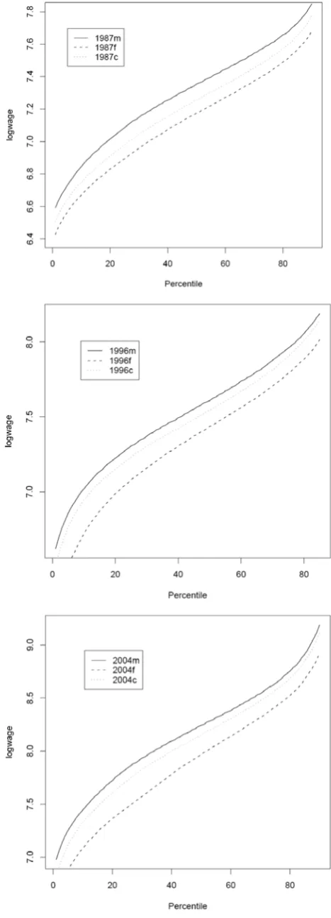
To show gender differences in pay across the wage distribution, we plot kernel

density estimates of earnings distribution for men and women in 1987, 1996, and

2004 (Figure 1). The logarithm of earnings is taken. From the kernel density estimates,

we recover gender differences in log earnings at different quantiles. These figures

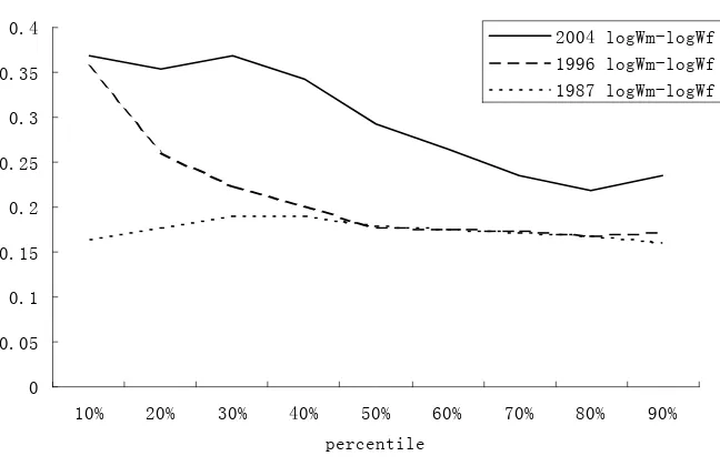
give estimates of the raw gender pay gap, as plotted in Figure 2. As it can be seen, in

1987 the gender pay differentials were similar across the distribution. In 1996, the

gender pay gap at the upper half of the distribution remained roughly the same as

1987, while that at the lower half of distribution increased disproportionally, resulting

in a much wider gender pay gap at the bottom. In 2004, the gender pay differentials

increased across the distribution but the increase was still much larger at the lower

quantiles. These findings are preliminary evidence supporting the emergence of the

“sticky floor” in China.

3. Methods

The empirical methods used in this study come mainly from Firpo, Fortin, and

Lemieux (2005, 2006). At the core of these methods is an unconditional quantile

regression (RIF projection).

3.1 Unconditional quantile (UQ) regression/RIF projection

Regression models establish conditional relationships between a response variable

Y and a set of explanatory variables X. However, many questions of economic and

policy interest concern the influence of X on the unconditional statistics of Y. For

(13)

12

is on earnings in a given population that contains individuals with different

characteristics (unconditional effects), rather than the impact just for a subgroup with

specific covariates (conditional effects). As far as the mean is concerned, the

unconditional properties of Y can be easily obtained by averaging it over X. This is

because linear regression models have a classical property, i.e. conditional mean

modelE Y X( | )=Xβ leads to ( | )E Y X =E X( )β immediately. Nevertheless, this

convenience hinges on the linearity of the expectation operator and hence cannot be

generalized to cases with nonlinear operators such as quantiles, i.e., the conditional

quantile regression models cannot answer questions about the unconditional statistical

properties of the response variable Y. The quantile regression method developed by

Koenker and Bassett (1978), which is commonly used in past research, is in fact a

conditional quantile regression. In contrast, the RIF method proposed by Firpo, Fortin,

and Lemieux (2006) is an unconditional quantile (UQ) regression.

Let ν be a distributional statistic of interest, in our case, a quantile. The

influence function (IF) of ν at point y in robust statistics and econometrics is

defined as:

, ,

0

( ) ( ) ( ) ( ; , ) lim t y t y

t

F F F

IF y F

t t

ν ν ν

ν Δ Δ

↓

=

− ∂

≡ =

∂ (1)

where Ft,Δy = −(1 )t F+ Δt y is a slight perturbation of F by point mass at y.

The recentered influence function (RIF) is obtained by adding the original

quantile back to its IF:

( ; , ) ( ) ( ; , )

RIF yν F ≡ν F +IF yν F . (2)

For example, RIF for a quantile q_τ is given by:

( )

( ; )

( ) Y I Y q RIF Y q q

f q

τ

τ τ

τ

τ− ≤

(14)

13

where fY is the marginal density function of Y, and ( )I ⋅ an indicator function.

Let GY be the counterfactual distribution of Y, obtained by replacingFX( )x

with another distribution GX( )x while keeping the conditional distribution

| ( )

Y X

F ⋅ unchanged,

|

( ) ( | ) ( )

Y Y X X

G y =

∫

F y X =x dG x . (4)

Central to the UQ regression method is the following observation (Theorem 1 in Firpo

et al, 2005):

[

]

, , , , 0 0 ( ) ( ) ( )

( ) lim

= ( ; ) ( )( )

= ( ; ) | ( )( )

Y t G

Y t G G t t Y Y X X F F F t t

RIF y d G F y

E RIF Y X x d G F x

ν ν ν π ν ν ν ↓ = − ∂ = = ∂ − = −

∫

(5)

which manifests that the marginal effects of the covariates on the unconditional

quantiles can be obtained by averaging the RIF-regression E RIF Y

[

( ; ) |ν X =x

]

with respect to the change in the distribution of the covariates, (d GX −FX). One can

further derive the unconditional partial effects of the covariates:

I. [Continuous covariate]: ( ) dE RIF Y

[

( ; ) | X x

]

dF x( )

dx ν

α ν =

_∫

= (6)

II. [Dummy covariate]:

[

] [

]

( ) ( ; ; ) | 1 ( ; ; ) | 0

D E RIF Y F X E RIF Y F X

α ν = ν = − ν = (7)

For estimation purpose, we apply the RIF regression in Firpo et al (2006). We first

estimate the RIF by replacing the unknown quantities by their estimators respectively:

n

l ( )

( ; )

( ) Y I Y q RIF Y q q

f q

τ

τ τ

τ

τ − ≤

= + , (8)

where q_τis the τth sample quantile, and lf_Y the kernel density estimator. Then we

use the familiar OLS method to fit the RIF-regression E RIF Y q

[

( ; ) |_τ X

]

with the

(15)

14

[

( ; ) |

]

E RIF Y q_τ X =Xβ . (9)

In this case, the partial effects of the covariates in (6) and (7) are given by the RIF

regression coefficients, β. Since the true RIF Y q( ; )_τ is unobservable, we use its

sample analogy nRIF Y q( ; )_τ in (9).

3.2 Counterfactual Distribution and Decomposition

A crucial question in the study of the gender wage gap is to separate the

endowment effect, i.e. the pay differences due to men and women’s different labor

market characteristics, from the discrimination effect, i.e. the pay differences as a

result of differences in the return to these characteristics. The well-known

Oaxaca-Blinder technique applies to the decomposition of the mean wage differences

between men and women, which follows immediately from the OLS estimates, but

does not work for other distributional statistics such as quantiles. To solve this

problem, many authors have developed decomposition methods for the entire wage

distribution. Several popular ones include: a reweighting method, which essentially

generates a counterfactual wage distribution (DiNardo, Fortin, and Lemieux, 1996;

Lemieux, 2002); an alternative approach based on conditional quantile regressions

and resampling (Machado and Mata, 2005; Autor, Katz, and Kearney, 2005; Melly,

2005, 2006); and another approach using semiparametric hazard functions to obtain

the conditional densities of wage (Donald, Green, and Paarsch, 2000).

The decomposition method that we use follows from Firpo, Fortin and Lemieux

(2005). This method consists of two steps. The first step resembles DiNardo et al

(1996) that decomposes the overall changes or differences between the two wage

distributions to those changes due to differences in characteristics and in the return to

(16)

15

decompose the differences between male and female wage at a quantile,

( )Ym ( )Yf

ν −ν , into the two components mentioned before, we produce a

counterfactual wage Yc, which represents the (log) wage that women could have

earned had they received the same return to their labor market characteristics as men.

Having done that, the overall difference ( )ν Ym −ν( )Yf can be decomposed into:

( )Ym ( ) [ ( )Yf Ym ( )] [ ( )Yc Yc ( )]Yf

ν −ν = ν −ν +ν −ν , (10)

where ( )ν Ym −ν( )Yc represents the endowment effect and ( )ν Yc −ν( )Yf represents

the discrimination effect. The counterfactual wage Yccan be obtained by reweighting.

We define the reweighting factor as

[

(1 ( )) / ( )

] [

/(1 )

]

i p Xi p Xi p p

ψ = − × − , (11)

where ( )p X is “the probability of a worker being a male given individual attributes

X” and p denotes the proportion of males in the population. Then the reweighted data

m Y

ψ can be regarded as realizations from the counterfactual wage distribution Yc. In

practice, ( )p X , which may be regarded as the “propensity score”, can be estimated

by the usual logit/probit model.

In the second step, the endowment effect and the discrimination effect are further

decomposed to the contribution of each individual covariate, as it is usually done with

the Oaxaca-Blinder composition. We note that the Machado-Marta approach can also

be used for the same purpose. Nevertheless their method entails multiple resamplings

and hence is computationally intensive. For each year, using the RIF-projection

method (9), we estimate the contribution of each explanatory variable to the

unconditional quantiles of male, female and counterfactual wages, which permits the

further decomposition of the contribution of each X variable to the two effects.

(17)

16

( )k ( k) ,k , ,

q Y_τ =E X β k =m f c (12)

where the subscripts m, f, c represent male, female and counterfactual respectively.

(12) is estimated by

_{( )} _kl _, _{, ,}

k k

q Y_τ =X β k=m f c, (13)

from which it follows the decomposition of the gender pay differences at a quantile

attributable to a specific X variable as following:

_{( )}_m _{( )}_f m₍l_m l_c_{) (} ml_c fl_f₎

q Y_τ −q Y_τ =X β −β + X β −X β . (14)

4. Results

4.1 RIF Pooled Regression with Gender Dummy

As shown in the descriptive results (Table 1), men and women had different labor

market characteristics. We begin by investigating into the extent which gender pay

differentials at different points of distribution may be explained by men and women’s

different characteristics. The pooled regressions with gender dummies are estimated

for 10th, 20th… up to 90th quantiles using the RIF method. The pooled regressions

impose the restriction that men and women receive the same return to a labor market

characteristic. Consequently, the coefficient estimate of gender dummy indicates the

gender gap that remains unexplained after controlling the individuals’ characteristics.

To see how much of the observed raw gender pay gap can be explained by various

characteristics, we conduct stepwise regressions. The list of control variables used in

each step can be seen in Table 3. For the purpose of brevity, only the estimates of

gender dummies are reported. The complete estimates of the model with the full set of

control variables (the last row under each year in Table 3) are reported in Appendix

Table 1a, Table 1b, and Table 1c for 1987, 1996, and 2004 respectively.

(18)

17

variables, the results suggest that the unexplained gender pay gap varies between 8-10

percent across the distribution in 1987. The gender pay gap increased rapidly in the

later years. The unexplained gap ranged between 11-34 percent in 1996 and 17-32

percent in 2004. It also appears that the gender pay gap became much wider at lower

quantiles in 1996 and 2004, suggesting that a “sticky floor” has emerged in China.

The evident inter-quantile differences also justify the use of RIF (unconditional

quantile regressions) rather than OLS. To test whether the pooled estimation is

appropriate, we interact all explanatory variables with the gender dummy and conduct

a Wald test. The result is significant at the one percent level, suggesting that the return

to labor market characteristics such as education attainment is significantly different

between men and women. This also implies that the estimations should be done for

each gender separately.

4.2 Separate RIF Regressions for Men and Women

Table 4a, Table 4b, and Table 4c show the RIF estimates for men and women

at the 10th, 50th, and 90th quantiles for 1987, 1996, and 2004 respectively. Except for

the 10th quantile in 1986 and 2004, the return to a one-year increase in work

experiences was greater for women than men. Compared to the return to the education

at a junior high level or below, return to college and high school education was also

greater for women than men. On the other hand, a lower return is found for women

working in private, foreign or joint-venture enterprises than state-owned or collective

enterprises and for female production and manual workers than white-collar

professional and managerial employees. Over time, these patterns did not diminish

but rather strengthened.

(19)

18

Since men and women had different labor market characteristics and also

differences in the return to these characteristics, we decompose gender pay

differentials to those explained by male-female different characteristics (also referred

to as the “endowment effect”) and those due to differences in the return to their

similar characteristics (also known as the “unexplained gap” or the “discrimination

effect”). As we explained in section 3, there are several approaches to decompose

differences between two distributions. We adopt the semi-parametric method

developed by Dinardo, Fortin, and Lemieux (1996), and extended by Lemieux (2002)

and Firpo, Fortin, and Lemieux (2005). At the center of this method, we construct a

counterfactual distribution using the “reweighting” technique. For each year, we

construct the counterfactual distribution of earnings that women could have earned

had they received the same return to a labor market characteristic as men. Men and

women’s actual distribution and the counterfactual distribution (denoted as “1987c,”

“1996c,” and “2004c”) are shown in Figure 3.

The differences between men’s actual wage distribution and the women’s

counterfactual represent the gender pay gap due to the endowment differences; the

differences between women’s actual distribution and the counterfactual indicate the

unexplained gap resulting from gender differences in the return to labor market

characteristics or the discrimination effect. As it can be seen, the discrimination effect

increased considerably from 1987 to 1996 and 2004. In fact, it accounted for more

than half of the raw gap in 1996 and 2004. To show the decomposition results more

clearly, Table 5 shows the explained and unexplained gender pay gap at mean and the

10th, 20th, …to 90th quantiles. Over time, the mean gender pay gap increased

(20)

19

pay gap potentially due to discrimination. From 1996 to 2004, the gender pay gap

continued to increase but the proportion of unexplained component did not

significantly increase further. Across the distribution, the overall gender pay gap and

the subcomponents were similar at different quantiles in 1987, while they became

quite different in 1996 and 2004. Specifically, they were greater at the lower quantiles

than the upper quantiles, lending strong support to the “sticky floor” hypothesis.

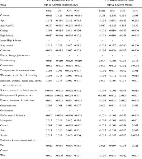
4.4 Decomposition with RIF

Using RIF, we further decompose the endowment effect and the discrimination

effect to the contribution of each explanatory variable. The results are documented in

Table 6a, Table 6b, and Table 6c for 1987, 1996, and 2004 respectively. If an

explanatory variable is a dummy variable, the estimate should be interpreted as the

relative contribution of this specific variable to the base group. In all the three years,

gender differences in work experiences, college education attainment, ownership type

of employers, and the likelihood of working in the manufacturing industry and

managerial occupation constitute a large portion of the endowment effect.

On the other hand, since the return to employment experiences and the return to

college and high school education attainment (relative to that of junior high level or

below) were higher for women than men, these variables actually equalize the pay

between men and women rather than widen the gap. As shown in the earlier results

(Table 4a, Table 4b, and Table 4c), women were paid a lower wage especially in

private, foreign or joint venture companies (the base group) than in state-owned or

collective companies. This leads to the results in Table 6a, Table 6b, and Table 6c,

which show that the estimates for the state and collective enterprises are negative,

(21)

20

sectors contribute less to the overall discrimination effect than the base group, i.e.

different returns in the private, foreign or joint venture companies.

Similarly, earlier results (Table 4a, Table 4b, and Table 4c) show that relative to

men, women who worked as production and manual laborers (the base group)

received a lower pay than those in professional and clerical jobs. Accordingly, the

results in Table 6a, Table 6b, and Table 6c, show that the male-female differences in

the return to professional and clerical occupations contribute less to the discrimination

effect than the different returns to male and female manual laborers. Overall, the

results suggest that the gender pay discrimination comes mostly from discrimination

against women who were less educated, blue-collar production workers working in

private, foreign, or joint venture companies.

5. Summary and Conclusion

Using a representative sample of national data for 1987, 1996, and 2004, we

examine the evolution of gender pay gap across the wage distribution in China. We

found that the overall gender pay gap and the component due to gender differences in

the return to labor market characteristics (the discrimination effect) had increased

substantially from 1987 to 1996 and 2004. The increase was greater for lower

quantiles than upper quantiles, hence the raw gender pay gap and the gap due to

discrimination became much wider at the bottom of wage distribution. We interpret

this as evidence of the “sticky floor” effect.

Using the RIF projection, we further decompose the gender pay gap and the

explained and unexplained components into the contribution of each individual

variable. The gender differences in years of work experiences, college education

(22)

21

positions contributed most to the explained gap. By contrast, the lower return to

women who only had junior high or lower levels of education and worked as

production and manual laborers in private, foreign or joint venture enterprises

accounts for most of the unexplained gap. Our study thus posits that women,

especially those low-wage earners who have had relatively less education, working as

(23)

22

References:

Adamchik, Vera A., Arjun S. Bedi. (2003) “Gender Pay Differentials During the

transition in Poland.” Economics of Transition, 11 (4): 697-726.

Albrecht, James, Anders Björklund, Susan Vroman. (2003) “Is There a Glass Ceiling

in Sweden?” Journal of Labor Economics, 21(1): 145-77.

Arulampalam, Wiji, Alison L. Booth, Mark L. Bryan. (2007) “Is There a Glass Ceiling over Europe? Exploring the Gender Pay Gap across the Wage Distribution.” Industrial and Labor Relations Review, 60(2): 163-86.

Autor, David H, Lawrence F. Katz, Melissa S. Kearney. (2005) “Rising Wage Inequality: the Role of Composition and Prices.” NBER working paper 11628

Becker, G. (1971). The Economics of Discrimination (2nd ed.). Chicago: University

of Chicago Press.

Blau, Francine D., Lawrence M. Kahn. (2006) “The US Gender Pay Gap in the 1990s: Slowing Convergence.” Princeton University, Industrial Relations Section, Working Paper #508

Booth, Alison L., Marco Francesconi, Jeff Frank. (2003) “A Sticky Floors Model of

Promotion, Pay, and Gender.” European Economic Review, 47(2): 295-322.

De la Rica, Sara, Juan J. Dolado, and Vanesa Llorens. (2005) “Ceiling and Floors:

Gender Wage Gaps by Education in Spain.”Bonn, Germany: IZA Discussion

Paper No. 1483

Del Río, Coral, Carlos Gradín, Olga Cantó. (2006) “The Measurement of Gender Wage Discrimination: The Distributional Approach Revisited.” ECINEQ Working Paper 2006-25

Dé_{murger, Sylvie, Martin Fournier, Yi Chen. (2005) “The Evolution of Gender}

Earnings Gaps and Discrimination in Urban China: 1988-1995.” Mimeo, University of Hongkong and CNRS

DiNardo, John, Nicole M. Fortin, Thomas Lemieux.(1996) “Labor Market Institutions

and the Distribution of Wages, 1973-1992: A Semiparametric Approach.”

Econometrica, 64(5): 1001-44.

Donald S, Green D, Paarsch H. (2000). “Differences in the Wage Distributions between Canada and the United States: an Application of a Flexible Estimator of the

Distribution Function in the Presence of Covariates.”Review of Economic Studies (67):

609-33.

(24)

23

Emerging Industrial Labor Market.” China Economic Review, 13 (2002) 170-96.

Dong, Xiao-yuan, Fiona Macphail, Paul Bowles, and Samuel P.S. Ho.(2003) “Gender Segmentation at Work in China’s Privatized Rural Industry: Some Evidence from

Shandong and Jiangsu.” World Development, 32(6): 979-98.

Firpo, Sergio, Nicole M. Fortin, Thomas Lemieux. (2005) “Decomposing Wage Distributions using Influence Function Projections.” Mimeo, Department of Economics, University of PUC-RIO.

Firpo, Sergio, Nicole Fortin, Thomas Lemieux. (2006) “Unconditional Quantile Regressions.” Mimeo, Department of Economics, University of PUC-RIO.

Gustafsson, BjoÈrn, Shi Li. (2000) “Economic Transformation and the Gender

Earnings Gap in Urban China.” Journal of Population Economics, 13:305-29.

Koenker R, Bassett G. (1978) “Regression quantiles.” Econometrica 46: 33–50.

Kee, Hiau Joo. (2006) “Glass Ceiling or Sticky Floor? Exploring the Australian

Gender Pay Gap.” The Economic Record, 82(259): 408-27.

Lemieux, Thomas.(2002) “Decomposing Changes in Wage Distributions: a Unified

Approach.” Canadian Journal of Economics, 35(4): 646-88.

Liu, Amy Y.C. (2004) “Gender wage gap in Vietnam: 1993 to 1998.” Journal of

Comparative Economics, 32:586-96.

Liu, Pak-Wai, Xin Meng, Junsen Zhang. (2000) “Sectoral Gender Wage Differentials

and Discrimination in the Transitional Chinese Economy.” Journal of Population

Economics, 13: 331-52.

Machado José A.F. and José Mata. (2005) “Counterfactual Decomposition of Changes

in Wage Distributions Using Quantile Regression.” Journal of Applied Econometrics,

20: 445-65.

Maurer-Fazio, Margaret, Thomas G. Rawski, Wei Zhang. (1999) “Inequality in the Rewards for Holding up Half the Sky: Gender Wage Gaps in China's Urban Labour

Market, 1988-1994.”The China Journal, 41: 55-88.

Maurer-Fazio Margaret, James Hughes. (2002) “The Effects of Market Liberalization

on the Relative Earnings of Chinese Women.” Journal of Comparative Economics,

30:709-31.

Melly, Blaise.(2005) “Decomposition of Differences in Distribution using Quantile

Regression.” Labour Economics, 12: 577-90.

(25)

24

Regression.” Mimeo, Swiss Institute for International Economics and Applied Economic Research (SIAW), University of St. Gallen.

Meng Xin, Paul Miller. (1995) “Occupational Segregation and Its Impact on Gender

Wage Discrimination in China's Rural Industrial Sector.” Oxford Economic Papers,

New Series, 47(1): 136-155.

Meng, Xin. (1998a). “Gender Occupational Segregation and its Impact on the gender

Wage Differential Among Rural-Urban Migrants: a Chinese Case Study.” Applied

Economics, 30: 741-52.

Meng, Xin. (1998b) “Male–female Wage Determination and Gender Wage

Discrimination in China’s Rural Industrial Sector.” Labour Economics, 5: 67–89.

Pham, T. Hung, Barry Reilly. (2006)“The Gender Pay Gap in Vietnam, 1993-2002:A Quantile Regression Approach.” PRUS Working Paper No.34

Reilly, Barry. (1999). “The gender pay gap in Russia during the transition, 1992–96.” Economics of Transition, 7 (1): 245-64.

Rozelle, Scott, Xiao-Yuan Dong, Linxiu Zhang, Andrew Mason. (2002) “Gender Wage Gaps in Post-Reform Rural China.” Working Paper, The World Bank Development Research Group.

Wang, Meiyan, Fang Cai. (2005). “Gender Wage Differentials in China’s Urban Labor Market.” Working Paper, Institute of Population and Labor Economics, Chinese Academy of Social Science.

(26)

[image:26.595.87.519.75.724.2]

25 Table 1: labor Market Characteristics by Gender, 1987-2004

1987 1996 2004

Male Female Male Female Male Female

Age 38.82 35.68 40.06 37.66 42.31 39.43

Education

College 14.56 6.08 26.51 15.3 36.88 31.29

High School 34.52 35.83 40.76 47.65 37.88 45.41

Junior High & Below 50.92 58.09 32.73 37.04 25.24 23.3

Industry

100% 100% 100% 100% 100% 100%

Manufacturing 39.93 43.63 38.7 37.75 25.06 20.98

Construction 4.32 2.84 3.7 2.51 3.90 1.88

Transportation & communication 7.82 4.13 7.19 4.26 11.42 5.82

Wholesale, retail, food & boarding 11.01 17.34 12.18 17.93 10.34 17.28

Education, cultural, health care, sports, and

social service

10.06 13.78 10.28 14.50 10.13 15.08

Science, research, technical service 2.69 1.58 2.96 2.15 2.88 2.72

Other personal and private service 1.96 2.85 3.75 5.01 8.57 12.71

Finance, insurance & real estate 1.85 2.02 2.41 2.35 4.68 5.87

Government 14.78 7.13 16.1 10.9 15.05 12.69

Other 5.60 4.70 2.74 2.64 7.97 4.97

Occupation

100% 100% 100% 100% 100% 100%

Professional & Technical 15.77 16.37 21.85 24.42 19.49 20.77

Managerial 13.84 2.96 11.49 3.07 7.03 2.25

Clerical 21.97 19.76 21.94 21.89 30.46 30.31

Sales 4.43 9.67 4.74 9.5 3.87 8.71

Service 2.84 8.59 2.51 6.4 8.14 17.22

Production and other manual workers 41.14 42.64 37.46 34.71 31.01 20.75

Ownership

100% 100% 100% 100% 100% 100%

State-owned 84.29 69.53 84.6 74.11 71.13 60.56

Collective 14.17 28.04 9.16 18.1 5.29 8.57

Private or self-employed 0.84 1.21 2.65 2.77 8.91 9.96

Foreign or Joint venture 0.7 1.22 3.59 5.01 14.67 20.91

Region

100% 100% 100% 100% 100% 100%

East 40.65 40.92 42.64 42.9 49.14 48.75

Central 34.43 34.16 35.72 35.33 31.53 31.57

West 24.92 24.92 21.64 21.77 19.33 19.69

100% 100% 100% 100% 100% 100%

(27)

[image:27.595.88.537.54.724.2]

26 Table 2: Descriptive Gender Pay Gap, 1987-2004

1987 1996 2004

Male Female F/M Female Male F/M Male Female F/M Mean Earnings 1546.52 1294.05 84% 2189.26 1793.85 82% 4215.07 3203.51 76%

Mean Earnings by Age Group

Age 16-25 966.24 926.50 96% 1374.02 1335.55 97% 2682.18 2498.88 93%

Age 26-35 1387.04 1257.62 91% 1979.39 1703.11 86% 3955.35 3219.52 81%

Age 36-45 1636.97 1410.91 86% 2306.51 1931.79 84% 4414.27 3309.49 75%

Age 46-55 1866.93 1538.59 82% 2461.39 2002.97 81% 4291.34 3246.32 76%

Age 56-65 1917.08 1446.32 75% 2482.00 1099.14 44% 4563.85 2583.26 57%

MeanEarnings by Education

College 1770.59 1591.47 90% 2500.13 2190.15 88% 5315.99 4352.00 82%

High School 1479.96 1306.76 88% 2098.73 1825.61 87% 3811.18 2942.00 77%

Junior High & Below 1527.59 1255.10 82% 2050.20 1589.28 78% 3212.95 2170.53 68%

MeanEarnings by Industry

Manufacturing 1488.50 1280.75 86% 2096.24 1703.32 81% 3701.59 2754.42 74%

Construction 1618.07 1354.88 84% 2225.55 1682.39 76% 3689.35 2974.13 81%

Transportation & communication 1606.54 1327.47 83% 2568.81 2104.35 82% 4334.76 3598.77 83%

Wholesale, retail, food & boarding 1414.73 1220.29 86% 1981.43 1675.75 85% 3336.80 2464.24 74%

Education, cultural, health care, sports,

and social service

1661.26 1413.56 85% 2329.87 2043.27 88% 4951.63 4211.95 85%

Science, research, technical service 1781.86 1461.99 82% 2360.31 1948.83 83% 5697.20 4500.68 79%

Other personal & private service 1503.57 1172.59 78% 2473.32 1712.79 69% 3634.17 2470.69 68%

Finance, insurance & real estate 1530.25 1332.76 87% 2624.95 2221.98 85% 4770.25 3578.59 75%

Government 1617.43 1370.55 85% 2165.99 1873.72 87% 4889.30 3759.53 77%

Other 1594.66 1157.64 73% 2034.64 1442.05 71% 4609.42 3534.31 77%

Mean Earnings by Occupation

Professional & Technical 1750.16 1498.04 86% 2428.29 2096.57 86% 5193.23 4377.73 84%

Managerial 1857.42 1726.93 93% 2589.91 2492.16 96% 5604.47 4627.16 83%

Clerical 1533.71 1369.61 89% 2179.06 1912.85 88% 4708.97 3707.44 79%

Sales 1252.07 1190.36 95% 1756.67 1548.89 88% 2665.16 2092.98 79%

Service 1367.64 1152.28 84% 2062.19 1599.18 78% 2752.80 2193.53 80%

Production and other manual workers 1414.74 1202.76 85% 1996.15 1546.90 77% 3437.32 2505.98 73%

Mean Earnings by Ownership

State-owned 1583.00 1364.69 86% 2205.98 1907.68 86% 4547.38 3734.50 82%

Collective 1301.72 1134.37 87% 1698.52 1366.11 80% 3048.64 2414.90 79%

Private or self-employed 1778.82 1190.33 67% 2606.07 1683.07 65% 2474.18 1730.16 70%

Foreign or Joint venture 1832.04 1040.20 57% 2738.84 1717.07 63% 4082.12 2690.92 66%

Mean Earnings by Region

East 1616.95 1389.13 86% 2683.08 2169.10 81% 4919.98 3596.90 73%

Central 1458.46 1198.53 82% 1797.52 1477.77 82 % 3518.30 2780.39 79%

West 1553.31 1268.88 82% 1863.00 1567.22 84% 3559.93 2785.33 78%

Source: NBSC Urban Household Survey, 1987, 1996, and 2004

(28)

[image:28.595.97.328.68.721.2]

27 Figure 1: Kernel Density Estimates of Log Earnings Distribution by Gender in 1987-2004

(29)

[image:29.595.103.427.109.319.2]

28 Figure 2: Raw Gender Pay Gap by Quantile, 1987-2004

0 0.05 0.1 0.15 0.2 0.25 0.3 0.35 0.4

10% 20% 30% 40% 50% 60% 70% 80% 90%

percentile

2004 logWm-logWf 1996 logWm-logWf 1987 logWm-logWf

(30)

[image:30.595.85.544.70.660.2]

29 Table 3: Pooled Unconditional Quantile Regression/RIF Projection Estimates with Gender Dummy, 1987-2004

1987 10th 20th 30th 40th 50th 60th 70th 80th 90th OLS-mean

Observed Raw Gender Gap 0.164 0.178 0.191 0.190 0.180 0.176 0.172 0.169 0.162 0.179 Gender gap with control for age and

education

0.128 0.136 0.130 0.131 0.122 0.121 0.115 0.109 0.100 0.124

Gender gap with control for age, education, and ownership type

0.099 0.110 0.106 0.110 0.105 0.107 0.103 0.100 0.095 0.106

Gender gap with control for age, education, ownership type, industry and occupation

0.093 0.098 0.094 0.097 0.093 0.092 0.089 0.086 0.078 0.093

Gender gap with control for age, education, ownership type, industry and occupation, and region

0.093 0.098 0.093 0.097 0.093 0.092 0.090 0.086 0.078 0.093

1996

education

0.339 0.228 0.185 0.154 0.138 0.132 0.123 0.125 0.132 0.182

0.286 0.193 0.157 0.131 0.119 0.116 0.111 0.118 0.131 0.161

0.294 0.197 0.158 0.129 0.116 0.109 0.103 0.111 0.120 0.160

0.296 0.198 0.159 0.130 0.118 0.111 0.104 0.113 0.122 0.160

2004

education

0.366 0.334 0.357 0.294 0.247 0.214 0.186 0.184 0.180 0.255

0.319 0.291 0.310 0.254 0.215 0.188 0.166 0.170 0.172 0.223

0.277 0.259 0.281 0.238 0.204 0.179 0.159 0.163 0.163 0.201

0.276 0.258 0.280 0.236 0.202 0.177 0.158 0.160 0.160 0.200

(31)

30 Table 4a: Unconditional Quantile Regression/RIF Projection Estimates for Male and Female Separately, 1987

RIF Estimates-Male RIF Estimates-Female

1987 10th 50th 90th 10th 50th 90th

Estimate Std. Error Estimate Std. Error Estimate Std. Error Estimate Std. Error Estimate Std. Error Estimate Std. Error

Constant 2.920 0.081 6.113 0.048 7.686 0.057 3.308 0.080 5.503 0.053 7.208 0.058

Age 0.171 0.004 0.045 0.002 -0.005 0.002 0.142 0.004 0.059 0.003 -0.003 0.003

Age*Age/100 -0.184 0.004 -0.034 0.003 0.019 0.003 -0.170 0.005 -0.059 0.004 0.019 0.004

College 0.045 0.022 0.030 0.013 0.102 0.015 0.083 0.029 0.076 0.019 0.225 0.021

High School 0.015 0.014 0.001 0.008 0.031 0.010 0.076 0.014 0.027 0.010 0.046 0.010

Junior High & Below - - - - - - - - - - - -

State-owned 0.128 0.049 -0.064 0.029 -0.246 0.035 0.474 0.041 0.195 0.027 -0.011 0.029

Collective -0.011 0.051 -0.156 0.030 -0.295 0.036 0.283 0.041 0.014 0.027 -0.102 0.030

Private, foreign, joint venture - - - - - - - - - - - -

Manufacturing -0.002 0.020 0.023 0.012 0.082 0.014 0.025 0.027 0.093 0.018 0.134 0.019

Construction -0.010 0.034 0.038 0.020 0.170 0.024 0.001 0.043 0.044 0.028 0.225 0.031

Transportation& communication 0.008 0.027 0.076 0.016 0.149 0.019 0.023 0.037 0.067 0.025 0.166 0.027

Wholesale,retail,food&boarding -0.076 0.027 -0.018 0.016 0.057 0.019 -0.029 0.031 -0.008 0.020 0.092 0.022

Education, cultural,health care,

sports, & social service

-0.004 0.046 0.011 0.027 0.078 0.033 0.018 0.044 -0.045 0.029 0.077 0.032

Science, research, technical service

-0.022 0.026 -0.008 0.015 0.041 0.018 -0.012 0.029 0.022 0.019 0.044 0.021

Other personal & private service -0.014 0.040 0.091 0.023 0.177 0.028 0.054 0.052 0.115 0.035 0.218 0.038

Finance, insurance& real estate 0.028 0.046 -0.043 0.027 0.091 0.032 0.096 0.047 0.028 0.031 0.134 0.034

Other industries -0.007 0.030 0.042 0.018 0.150 0.022 -0.194 0.037 -0.004 0.025 0.102 0.027

Government - - - - - - - - - - - -

Professional & Technical 0.051 0.023 0.074 0.014 0.052 0.016 0.075 0.023 0.137 0.015 0.087 0.017

Managerial 0.053 0.022 0.106 0.013 0.109 0.015 0.079 0.038 0.241 0.025 0.245 0.028

Clerical 0.060 0.018 -0.026 0.011 -0.008 0.013 0.094 0.019 0.098 0.013 0.043 0.014

Sales -0.085 0.035 -0.060 0.021 -0.030 0.025 0.023 0.029 0.054 0.019 0.019 0.021

Service -0.026 0.038 -0.053 0.023 -0.040 0.027 -0.111 0.025 0.010 0.017 0.011 0.018

Production & manual workers - - - - - - - - - - - -

East 0.092 0.014 0.087 0.008 0.096 0.010 0.132 0.014 0.115 0.009 0.126 0.010

Central - - - - - - - - - - - -

West 0.032 0.016 0.017 0.009 0.036 0.011 -0.004 0.016 -0.013 0.010 0.061 0.011

(32)

31 Table 4b: Unconditional Quantile Regression/RIF Projection Estimates for Male and Female Separately, 1996

1996 10th 50th 90th 10th 50th 90th

Constant 1.304 0.129 5.980 0.059 7.321 0.097 0.741 0.171 5.211 0.069 6.765 0.103

Age 0.248 0.006 0.056 0.003 0.037 0.005 0.271 0.009 0.086 0.004 0.044 0.006

Age*Age/100 -0.279 0.008 -0.053 0.004 -0.037 0.006 -0.346 0.012 -0.099 0.005 -0.049 0.007

College 0.196 0.030 0.143 0.014 0.151 0.023 0.217 0.044 0.175 0.018 0.195 0.026

High School 0.145 0.023 0.060 0.011 0.058 0.017 0.128 0.029 0.086 0.012 0.078 0.018

Junior High & Below - - - - - - - - - - - -

State-owned 0.170 0.042 -0.011 0.019 -0.396 0.031 0.421 0.050 0.132 0.020 -0.110 0.030

Collective -0.161 0.050 -0.227 0.023 -0.527 0.038 -0.021 0.055 -0.135 0.022 -0.283 0.033

Manufacturing -0.077 0.031 0.052 0.014 0.083 0.024 0.067 0.048 0.023 0.019 0.101 0.029

Construction -0.151 0.055 0.127 0.025 0.183 0.041 0.007 0.085 0.032 0.034 0.163 0.052

Wholesale, retail, food& boarding -0.172 0.041 0.008 0.019 0.104 0.031 0.010 0.055 -0.018 0.022 0.150 0.033

Education, cultural, health care,

sports, and social service

-0.018 0.054 0.109 0.025 0.231 0.041 -0.176 0.067 0.031 0.027 0.158 0.041

-0.033 0.039 0.075 0.018 0.086 0.029 0.086 0.051 0.083 0.021 0.119 0.031

Other personal & private service -0.025 0.059 0.072 0.027 0.152 0.044 0.076 0.090 0.003 0.036 0.064 0.054

Finance, insurance & real estate 0.106 0.064 0.275 0.030 0.309 0.048 0.229 0.086 0.230 0.035 0.350 0.052

Other industries -0.153 0.061 -0.078 0.028 -0.007 0.046 -0.420 0.084 -0.118 0.034 -0.022 0.051

Government - - - - - - - - - - - -

Managerial 0.237 0.037 0.152 0.017 0.142 0.028 0.442 0.078 0.332 0.031 0.339 0.047

Clerical 0.149 0.029 0.003 0.013 0.021 0.022 0.262 0.039 0.128 0.016 0.132 0.024

Sales -0.138 0.054 -0.071 0.025 -0.123 0.040 0.135 0.058 0.016 0.023 -0.020 0.035

Service -0.023 0.063 0.027 0.029 -0.042 0.047 0.019 0.056 0.055 0.023 0.048 0.034

Production &other manual workers - - - - - - - - - - - -

East 0.254 0.021 0.295 0.010 0.464 0.016 0.302 0.027 0.316 0.011 0.453 0.016

Central - - - - - - - - - - - -

West 0.030 0.025 0.021 0.012 0.005 0.019 0.101 0.033 0.060 0.013 -0.012 0.020

(33)

32 Table 4c: Unconditional Quantile Regression/RIF Projection Estimates for Male and Female Separately, 2004

2004 10th 50th 90th 10th 50th 90th

Constant 3.193 0.127 6.294 0.060 7.370 0.104 4.328 0.131 5.540 0.080 7.010 0.104

Age 0.155 0.006 0.064 0.003 0.040 0.005 0.094 0.007 0.083 0.004 0.048 0.005

Age*Age/100 -0.175 0.007 -0.065 0.003 -0.038 0.006 -0.110 0.008 -0.097 0.005 -0.050 0.007

College 0.320 0.023 0.303 0.011 0.398 0.019 0.367 0.024 0.466 0.014 0.405 0.019

High School 0.201 0.019 0.110 0.009 0.098 0.016 0.233 0.019 0.186 0.012 0.087 0.015

Junior high & below - - - - - - - - - - - -

State-owned 0.495 0.019 0.170 0.009 -0.018 0.015 0.316 0.018 0.304 0.011 0.125 0.015

Collective 0.133 0.035 -0.102 0.016 -0.159 0.028 0.182 0.028 -0.011 0.017 -0.056 0.022

Manufacturing -0.008 0.027 -0.173 0.013 -0.020 0.022 0.053 0.029 -0.150 0.018 -0.053 0.023

Construction -0.077 0.042 -0.147 0.020 -0.029 0.035 -0.100 0.057 -0.171 0.035 0.015 0.045

Wholesale, retail, food &boarding -0.189 0.034 -0.141 0.016 -0.033 0.028 -0.118 0.032 -0.104 0.019 0.072 0.025

Education, cultural, health care,

sports, and social service

-0.238 0.032 -0.129 0.015 -0.049 0.026 -0.231 0.030 -0.226 0.018 -0.033 0.024

-0.016 0.031 0.035 0.015 0.051 0.025 0.017 0.030 0.071 0.018 0.142 0.024

Other personal & private service 0.062 0.047 0.114 0.022 0.272 0.038 0.016 0.049 0.131 0.030 0.269 0.039

Finance, insurance & real estate 0.042 0.039 -0.016 0.018 0.139 0.032 0.022 0.036 0.011 0.022 0.229 0.029

Other industries 0.086 0.033 0.065 0.015 0.227 0.027 0.097 0.039 0.061 0.024 0.172 0.031

Government - - - - - - - - - - - -

Managerial 0.296 0.034 0.251 0.016 0.294 0.028 0.328 0.053 0.413 0.033 0.324 0.043

Clerical 0.277 0.022 0.136 0.010 0.144 0.018 0.288 0.025 0.273 0.015 0.128 0.020

Sales -0.422 0.045 -0.147 0.021 -0.035 0.037 0.008 0.037 -0.075 0.023 -0.094 0.029

Service -0.318 0.031 -0.142 0.014 -0.084 0.025 -0.018 0.028 -0.109 0.017 -0.072 0.022

Production& other manual workers - - - - - - - - - - - -

East 0.268 0.016 0.244 0.008 0.546 0.013 0.219 0.017 0.231 0.010 0.439 0.013

Central - - - - - - - - - - - -

West 0.010 0.021 0.034 0.010 0.017 0.017 0.016 0.021 0.100 0.013 0.047 0.016

(34)

[image:34.595.97.331.64.712.2]

33 Figure 3: Counterfactual Distribution and the Gender Pay Gap Decomposition, 1987-2004

(35)

[image:35.595.89.507.83.288.2]

34 Table 5: Decomposition of the Gender Pay Gap at Selected Quantiles, 1987-2004

1987 Mean 10th 20th 30th 40th 50th 60th 70th 80th 90th

Observed Raw Gap 0.179 0.164 0.178 0.191 0.190 0.180 0.176 0.172 0.169 0.162 Explained gap 0.082 0.085 0.099 0.106 0.106 0.099 0.092 0.092 0.085 0.078 Unexplained gap 0.097 0.080 0.079 0.086 0.084 0.081 0.084 0.080 0.084 0.084

1996

Observed Raw Gap 0.223 0.355 0.262 0.225 0.201 0.177 0.176 0.175 0.168 0.173 Explained gap 0.068 0.090 0.074 0.074 0.074 0.065 0.065 0.065 0.057 0.041 Unexplained gap 0.155 0.265 0.189 0.152 0.128 0.111 0.110 0.110 0.111 0.132

2004

(36)

[image:36.595.89.546.64.574.2]

35 Table 6a: Decomposition of the Gender Pay Gap to Specific Variables at Selected Quantiles, 1987

1987

The Endowment Effect due to different characteristics

The Discrimination Effect due to different returns

Mean 10% 50% 90% Mean 10% 50% 90%

Constant 0.078 0.545 -0.177 -0.113 0.261 -0.932 0.787 0.592

Age 0.101 -0.751 0.392 -0.008 -0.373 2.334 -0.770 -0.069

Age*Age/100 -0.193 0.176 -0.209 0.058 0.462 -0.864 0.455 -0.010

College 0.004 0.002 0.001 0.009 -0.002 -0.001 -0.001 -0.008

High School -0.003 -0.011 0.001 0.002 -0.010 -0.011 -0.010 -0.007

Junior High & below - - - - - - - -

State-owned 0.020 0.084 0.025 -0.015 -0.254 -0.306 -0.214 -0.185

Collective 0.040 0.026 0.033 0.042 -0.085 -0.107 -0.059 -0.055

Private, foreign, joint venture - - - - - - - -

Manufacturing 0.010 0.009 0.006 0.023 -0.035 -0.020 -0.038 -0.049

Construction 0.002 0.0003 0.0004 0.005 -0.001 -0.001 0.0004 -0.004

Transportation & communication 0.003 0.0004 0.003 0.008 -0.001 0.0003 0.0003 -0.003

Wholesale, retail, food & boarding 0.004 0.014 0.002 0.001 -0.007 -0.017 -0.003 -0.011

Education, cultural, health care, sports,

and social service

0.0004 0.002 0.0004 0.001 0.0004 -0.002 0.001 -0.001

Science, research, technical service 0.003 0.001 0.004 0.003 -0.005 -0.002 -0.008 -0.005

Other personal & private service 0.001 0.001 0.001 0.003 -0.001 -0.002 0.0004 -0.002

Finance, insurance & real estate 0.0003 0.0004 0.0003 0.001 -0.001 -0.001 -0.001 -0.002

Other industries 0.001 0.0004 0.001 0.005 0.003 0.009 0.002 -0.001

Government - - - - - - - -

Professional & Technical 0.003 0.002 0.003 0.008 -0.013 -0.006 -0.014 -0.014

Managerial 0.010 0.006 0.011 0.013 -0.003 -0.001 -0.004 -0.005

Clerical 0.001 0.007 -0.001 0.001 -0.017 -0.012 -0.024 -0.012

Sales 0.002 0.002 0.001 0.003 -0.009 -0.008 -0.009 -0.006

Service 0.002 0.002 0.002 0.002 -0.002 0.007 -0.004 -0.004

Production &other manual workers - - - - - - - -

East -0.006 -0.018 -0.009 0.008 -0.009 0.002 -0.003 -0.020

Central - - - - - - - -

West -0.002 -0.010 -0.002 0.002 0.004 0.019 0.009 -0.008