Munich Personal RePEc Archive
The Effect of Newer Drugs on Health
Spending: Do They Really Increase the
Costs?
Civan, Abdülkadir and Koksal, Bulent
Fatih University Department of Economics, Fatih University
-Department of Economics
October 2007
The Effect of Newer Drugs on Health Spending:
Do They Really Increase the Costs?
Abdülkadir Civan
Fatih University
Bülent Köksal
Fatih University
October 2007
Abstract. We analyze the influence of technological progress on pharmaceuticals on rising health expenditures using US State level panel data. Improvements in medical technology are believed to be partly responsible for rapidly rising health expenditures. Even if the technological progress in medicine improves health outcomes and life quality, it can also increase the expenditure on health care. Our findings suggest that newer drugs increase the spending on prescription drugs since they are usually more expensive than their predecessors. However, they lower the demand for other types of medical services, which causes the total spending to decline. A one-year decrease in the average age of prescribed drugs causes per capita health expenditures to decrease by $31.92. The biggest decline occurs in spending on hospital and home health care due to newer drugs.
JEL Classification Code: I10; I11; C23
Keywords: Health care expenditure; pharmaceuticals; technology diffusion.
1
1. Introduction
In most developed countries, there has been a rising trend in health expenditures. The
growth rates of the health expenditures are generally higher than the growth of the overall
economy. As a result, the ratio of the health expenditure to the GDP has been rising
continuously. The percentage of health expenditures in the GDP was 3.8% in 1960 for OECD
countries and has been continuously increasing since then.1. The trends in US and in most other countries have been similar. In the US, the ratio of health expenditures to the GDP rose
from 5.1% in 1960 to 15.3% in 2005. Moreover, there is a significant variation in health
expenditures among the relatively homogenous regions like OECD member countries or US
states. For example, while the UK devoted only 8.3% of her GDP to the health care in 2005,
the US spent almost twice.2 In the US, average per capita health expenditures for the period
1993-2004 ranged from $2,972 for Idaho to $8,738 for District of Columbia.3
This significant variation in health care spending begs an explanation. Different
societies might have different demand levels for health services or might have diverse health
care “needs” due to the differences in life style, environmental conditions, or genetic
characteristics. Alternatively, perhaps health care systems are not managed as efficiently as
possible everywhere. Health care markets are poised with numerous problems such as moral
hazard, principal-agent problems, and information failures. Any of these problems can cause
markets to operate inefficiently. When we look at the details of the health care spending, we
see that the inefficient management of health care systems is highly possible. For example,
pharmaceutical spending makes up only 9.4% of the total health expenditure in Norway,
while the same figure is 29.4% in Poland. Even if the variation in input choice for the health
care (production function) does not mean inefficiency per se, the size of this variation raises a
question mark. Indeed Baicker and Sandar (2004) and Fisher et al (2003a, 2003b) conclude
that higher spending in health care does not improve health outcomes or patient satisfaction
level. Thus, academics and policy makers have been analyzing the health care markets and
trying to understand the driving factors behind the continuing increase in health expenditures
for decades. In this paper, we contribute to the literature by analyzing the influence of
technological improvement in pharmaceutical markets on health spending levels using panel
data for US States.
1 The ratios of the health expenditures to the GDP for 1970, 1980, 1990, 2000 and 2004 were 5.0%, 6.7%, 6.9%,
7.9%, and 9.0%, respectively. These numbers are un-weighted averages of current OECD member countries
The rest of the paper is organized as follows: In section 2, we discuss some
background information and previous literature about the rising health expenditures. Section 3
summarizes the significance of pharmaceuticals on medical markets and on rising health
expenditures. Sections 4 and 5 present the data and empirical methodology, respectively. We
discuss the results in Section 6 and conclude in section 7.
2. Rise in Health Expenditures and New Technologies
Several explanations for the rising health expenditures have been cited in the health
economics literature. Primary explanation is the rising incomes. Wealthier individuals are
willing to pay more for their health, i.e. health care is a normal good. An increasing amount of
spending on health care is a natural result of economic growth. Almost all studies analyzing
the health care costs found a positive relationship between per capita income and health
spending.4 In fact, earlier studies conclude that income differences can explain almost all of the variation in the spending levels. Another reason for rising health spending is the aging
societies. Generally old and very old require much more health care than young and
middle-aged. Many studies use the percentage of population over 65 as a proxy for this demographic
shift. Most studies have concluded that aging societies are spending more on health services5. Insurance coverage is another explanation cited in the literature. As it is common in many
markets, insurance coverage can cause moral hazard problems. The individuals, who do not
pay for the whole costs of the services they get, tend to use more health care than the efficient
level. However, insurance firms are also better equipped than individual patients against the
health care suppliers. Specifically, they can use their market power to get favorable terms
because they can buy health services in bulk. Moreover, they can take much stronger
measures than the individual patients against the advantages of the suppliers due to
asymmetric information.
However, rising income levels, demographic shift and increased insurance coverage
can only explain a relatively small portion of the rise in health expenditures. Slade and
Anderson (2001) note that there is nearly a consensus among health economists that a
substantial portion of the increase in health care spending is due to diffusion of new medical
technologies. According to Newhouse (1992), usual suspects (supplier induced demand, aging
population, income growth, increased insurance) can explain approximately half of the rise in
the health expenditures. He conjectures that the rest of the increase should be given to
technological improvement in health services. Cutler et al. (1998) explains the significance of
the technological improvement on health spending with the following sentences:
“Nonetheless, it has now achieved a degree of acceptance, in part because it is difficult
to think of another factor that is common across six consecutive decades and across
many countries with different health-care financing institutions. Here we accept for
the sake of argument that a substantial portion of the spending rise is attributable to
the increased capabilities of medicine and ask what the spending increases-and
inferentially the increased capabilities-have bought.”
Cutler and Mcgellan (2001) classify the effects of new technologies into two groups:
They use the term “treatment substitution effects” to indicate that new technologies often
substitute for older technologies. The treatment costs of these new technologies maybe higher
or lower than old technologies. However, new technologies in medicine also make treatment
possible for patients who were not able to get treatment with old technologies. For example,
new surgical techniques made it possible to operate on very old patients. Cutler and Mcgellan
call this “treatment expansion effect”. They note that the diagnosis rates for depression
doubled after Prozac-like drugs became available, and cataract surgery was performed much
more frequently as the procedure improved. When the new treatment is effective, making it
available for more people is beneficial, but this would almost certainly increase the health
care spending.6 It is believed that the treatment expansion effect is a major factor in both the benefits of technological innovation and cost-increase.
Health economists usually presume that new technologies increase health
expenditures, because they are usually more expensive than the older technologies they
replace and they also expand the relevant market size, but the benefits are worth the extra
expense. Even posing the question of whether the new technologies are worth the extra cost
would be peculiar for other markets. Interactions of utility maximizing individuals and profit
maximizing firms would result in an equilibrium at which all questions are answered
automatically. However, even the most free-markets oriented economist would not claim that
the markets would make efficient allocation of resources in medical care.
6 However, it is also possible that a new technology might lower the overall health spending by substantially
The problems like moral hazard (patients pay only a fraction of the whole medical bill,
so they tend to overuse the medical services), supplier induced demand (suppliers have the
incentive and ability to increase the utilization of health services), principal-agent problem
(the interests of decision makers [generally doctors] do not coincide 100% with the principles
[hospitals, patients or insurance companies]), and asymmetric information (patients know
much less about their conditions and what would happen if they don’t listen to the doctor’s
recommendation) make it necessary to study the potential benefits and costs of new
technologies very carefully.
Hedonic methods have been used to measure the valuation of the new products and
technologies in many markets. However, usually customers of new technologies in health care
markets (patients) have insufficient information (one might say ignorant) about the effects of
new technologies. This makes it almost impossible to use hedonic techniques. Therefore,
most studies focus on the cost of new technologies in terms of higher spending and compare
these costs to the quantifiable health effects of the technologies, such as declines in mortality.
For example, Cutler and Mcgellan (2001) analyze new technologies in the treatment of five
conditions: heart attacks, low-birth weight infants, depression, cataracts and breast cancer.
They conclude that the estimated benefits of new technologies are much greater than the costs
for all conditions except breast cancer. The costs and benefits of the technological change in
breast cancer are approximately of equal magnitude.
3. Pharmaceuticals
Pharmaceuticals have been getting more attention than other types of medical services
for a number of reasons. First, the share of pharmaceutical spending on the total health
expenditures has been rising in the US and in many other OECD countries since 1980s. In the
US, the share of pharmaceutical drugs increased from historical lows of 8.7% in 1982 to
12.4% in 2005. Similarly, the share of pharmaceuticals on public agencies’ budgets has been
increasing. Duggan and Evans (2007) note that between 1995 and 2004, the fraction of
Medicaid costs on prescription drugs nearly doubled, from 7.4% to 13.7%. Most of this
increase was due to expensive new treatments. Average Medicaid prescription cost has risen
by 90% since 1995. Lichtenberg (2000) cites the Barents Group study for National Institute
for Health care Management (1999) which estimates that 42% of the drug costs between 1993
and 1998 were due to newer drugs costing more than older drugs. According to that study, the
compared to $30.47 for previously existing drugs. Naturally, the policymakers who are
desperate to implement cost-containment strategies have focused on pharmaceuticals.
Moreover, pharmaceutical drugs market is relatively concentrated with small number of large
multinational firms. So politically it is easier to focus on relatively few and very visible firms
than focusing on neighborhood doctors and hospitals.
Pharmaceutical companies have been very active on pushing “technological
improvement” on medical care. The pharmaceutical sector is one of the leading industries in
terms of R&D investment to revenue ratios. Drug companies use patents very effectively to
recover the fixed R&D costs. However, “monopolistic”7 structure of the market due to patents creates the perception that pharmaceutical companies are making excessive profits.8 Moreover, they make exaggerated claims about the merits of the new drugs for marketing
purposes. These claims coupled with the “insider stories” of “dirty secrets” of pharmaceutical
companies have created doubts about the value of the new drugs.
Like other types of technological improvements in the health care markets, newer
drugs can have ambiguous effects on the total health spending. Generally, newer drugs are
substantially more expensive than their predecessors and possibly, they would increase
overall spending. On the other hand, improvements in health outcomes due to their effective
use could reduce the need (or demand) for other types of medical care, such as hospital visits
and nursing home care, which could decrease the total spending on medical care.
Numerous studies have been published about the value of the new drugs. Most studies
focused on the effects of specific drugs on health outcomes and health expenditures. Hudson
et al (2003) surveys the papers studying the effect of the use of second-generation
antipsychotic medications health care costs. The majority of surveyed studies found that
second–generation antipsychotic drugs are either cost-neutral or reducing costs.
Duggan and Evans (2007) used the administrative data of Medicaid to estimate the
effect of antiretroviral drugs for HIV on health care spending and health outcomes. They
exploited the differential take-up of antiretroviral drugs at individual level. Their results
suggest that new drugs not only lower the mortality rate by 68% but they also decrease the
short-term health care spending by reducing expenditures on other categories of medical care.
The average lifetime Medicaid spending on AIDS patients has increased from $89,000 to
7 We do not claim that the drug companies are monopolies in technical sense. We mean that there is such a
perception.
$234,000, however, because AIDS patients live longer and require more medical care in the
long run.
Lichtenberg has published a series of articles on the values of new drugs using various
data sources and methodologies. His studies confirm the proposition that new drugs are not
only useful in terms of better health outcomes but they also lower the health expenditures.
Lichtenberg (1996) uses US data at disease level. He compares the health outcomes, health
expenditures and utilization of different health inputs (such as hospital admissions, physician
visits etc…) between 1980 and 1991. In addition, he analyzes the effects of using relatively
new drugs for different diseases on health outcomes and health expenditures. He concludes
that a $1 increase in pharmaceutical expenditure reduces total health care expenditures by
$2.65. In Lichtenberg (2001), he uses person-, condition-, and event-level data to study the
effect of drug age on total medical expenditure and mortality. Lichtenberg updates this study
using person condition level data in Lichtenberg (2002) which gives very similar results.
Lichtenberg (2006) focuses on HIV treatments using US national data for the period
1982-2001. He estimates that the increased utilization of HIV drugs increases the medical
care expenditures by $3,530 per AIDS patient, but it also increases the life expectancy of
AIDS patients by 13.6 years. Thus, the medical cost per additional life-year due to increased
utilization of HIV drugs is $17,175.9 However, this method does not allow for differential effectiveness of old and new HIV drugs. Presumably, the newer drugs are more effective on
lowering mortality and keeping patients out of hospitals. Thus, he concludes that $17,175 per
saved life-year is the upper bound for HIV drugs. However, in another study Duggan (2005)
finds that newer antipsychotic drugs have not reduced health spending. According to his
estimates, 610% increase in Medicaid spending on antipsychotic drugs has not reduced
spending on other types of medical care during 1993-2001 period. Thus, newer drugs have
increased total health costs.
The conclusions of the studies on the value of technological improvement and new
drugs have significant policy implications. If the new drugs are cost effective per saved
life-years, the policies that would reduce the pharmaceutical R&D should be evaluated very
carefully. Price regulations, allowing drug importations, putting restrictions on intellectual
property rights and other similar regulations are shown to be affecting pharmaceutical
companies’ R&D and marketing decisions10.
9 Lichtenberg (2006) notes that according to Murphy and Topel (2003), average value of US life-year is on the
order of $150,000.
Generally, patient/event/disease level data are used in the previous studies. These
studies try to control for the endogeneity of the drug use. Generally, newer drugs are first
prescribed and used on the patients who are relatively sicker than the average patient.
Therefore, their health care spending is higher than the average patient. Even though there
have been several approaches to consider this problem, we believe that the individual level
patient characteristics are very difficult to control. Thus in this study we are using state level
aggregate health spending data.11 More importantly using aggregate state level data allows us to analyze the treatment expansion effects of newer drugs. Studies that use disease level data
also encounter with spillover effects of the diseases. Certain diseases make the patients
vulnerable to other ones. Therefore, treatment of a disease might have extra benefits due to
spillover effects to other diseases. One should not overlook those crossover effects.
Moreover, we use a general proxy to determine the technological level of drugs: the number
of years passed since it was first approved by FDA. Most other studies selected specific drugs
and analyzed the effects of prescription patterns of these drugs on health spending12. Even if the choice of those drugs is far from arbitrary, relatively ad hoc character of this methodology
makes it harder to generalize the conclusions. Finally, we use US State level panel data unlike
most other studies on the health expenditure issue that use international (usually OECD) data.
As Wang and Rettenmaier (2006) point out, one advantage of US State data over international
data is that the US states are less heterogeneous in terms of health industry structure,
government policy, consumer preferences and payment mechanisms.
4. Data
We use annual data from 1993 to 2004 for 51 states in our estimations. Health Care
Expenditures (HCE) and Gross State Products (GSP) are from the webpage of the Center for
Medicare and Medicaid Services.13 We analyze the effect of technology on each of the following 11 categories reported by the Center for Medicare and Medicaid Services: Personal
health care, hospital care, physician and clinical services, other professional services, dental
services, home health care, prescription drugs, other non-durable medical products, durable
medical products, nursing home care, and other personal health care.14 We obtain state
11 One other advantage of the aggregate health spending data is that, it is less skewed than the patient level
spending.
12 Lichtenberg uses the same proxy in Lichtenberg (2001) 13http://www.cms.hhs.gov/
populations and GDP implicit price deflators to calculate the real per capita variables as well
as the percentage of the population over age 65 from the websites of the U.S. Census Bureau
and Bureau of Economic Analysis, respectively. We obtain insurance coverage data from U.S.
Census Bureau website. As stated there “private health insurance is coverage by a health plan
provided through an employer or union or purchased by an individual from a private health
insurance company, and the government health insurance includes plans funded by
governments as the federal, state, or local level. The major categories of government health
insurance are Medicare, Medicaid, the State Children’s Health Insurance Program (SCHIP),
military health care, state plans, and the Indian Health Service.” We make use of “Ambulatory
Health Care Data” from National Center for Health Statistics' web site15 to calculate the annual drug mentions for the period above.
Our key variable is the average drug age, which is a measure for the technological
progress in the market for drugs. To be more precise, we use the age of the active ingredients
of the drugs. A relatively lower average active ingredient age indicates newer technology. We
proceed as follows to calculate the average active ingredient age: First, we calculate the
annual drug mentions for each drug for our data period. Then, we calculate the total annual
mentions of each active ingredient. An active ingredient can appear more than once in
different drugs because of the combination drugs. Next, we match the names of these active
ingredients with the names of the active ingredients in FDA.16 FDA database has the first approval dates of the active ingredients, which we use to determine the ages of the active
ingredients. Once we have ages of the active ingredients, we calculate the weighted average
drug age as follows:
n
i=1
1
( )
i i
n i i
f Active Ingredient Age Drug Age
f
=
⋅ =
where fi is the total number of mentions and (Active Ingredient Age)i is the age of the
th
i active ingredient. Unfortunately, Ambulatory Health Care Data does not have the zip
codes for the drug mentions. Therefore, we were able to calculate the average drug age for
15http://www.cdc.gov/nchs/about/major/ahcd/ahcd1.htm
four US regions: Northeast, Midwest, South, and West.17 Accordingly, we assume that the average drug age is same for all states in the same region.
Table 1 reports the summary statistics for our data. Per capita health care expenditure
is $4024 while $382 of this amount is spent on prescription drugs. Average drug age varies
between 22.71 years and 23.80 years. Alaska is the youngest state and Florida is the oldest in
terms of the percentage of population over 65. Only 6% of Alaska residents are older than 65
while 18% of Floridians are older than 65. Insurance coverage also varies between states.
New Mexico has the lowest private insurance coverage with 57% and Iowa has the highest
with 82%. Average of government insurance coverage in US States is 26%.
5. Empirical Methodology
We estimate the following panel-data models:
1 2 3 4 5 65 6
it it it it it it i it
HCE =βDrugAge +β GSP +βGovIns +β PrivIns +β Over +β t+α +ε (1)
1 2 3 4 5 65
it it it it it it i it
HCE β DrugAge β GSP β GovIns β PrivIns β Over α ε
∆ = ∆ + ∆ + ∆ + ∆ + ∆ + + (2)
where i=1,...,51 and t=1,...,12; HCEit is per capita real health care expenditure for each
category mentioned in the previous section; Drug age is the weighted average age of the
active ingredients as described in the previous section; GSP is the per capita real gross state
product; GovIns and PrivIns are the government and private insurance coverage, respectively;
Over65 is the percentage of the population over age 65; αi is the unobserved state effect and
it
ε is the error term. Allowing for the time trend explicitly recognizes that HCE may be
changing over time for reasons unrelated to the exogenous variables that we use. Our purpose
is to analyze the long- and short-term effects of the new technology on HCE by estimating
equations 1 and 2, respectively.
As is well known, nonstationarity may be a problem for panel data especially when the
time dimension is long. Many papers in the earlier literature have found that the HCE and
GSP have unit-roots.18 We applied Levin-Lin-Chu19 test with time trend to HCE and GSP in
17
The states in each region are as follows. Northeast: Connecticut, Maine, Massachusetts, New Hampshire, New Jersey, New York, Pennsylvania, Rhode Island, Vermont; Midwest: Illinois, Indiana, Iowa, Kansas, Michigan, Minnesota, Missouri, Nebraska, North Dakota, Ohio, South Dakota, Wisconsin; South: Alabama, Arkansas, Delaware, District of Columbia, Florida, Georgia, Kentucky, Louisiana, Maryland, Mississippi, North Carolina, Oklahoma, South Carolina, Tennessee, Texas, Virginia, West Virginia; West: Arizona, California, Colorado, Idaho, Montana, Nevada, New Mexico, Oregon, Utah, Washington, Wyoming, Alaska, Hawaii
equation (1). The method described in Ng and Perron (2001) produces optimal lag lengths of
0, 1, or 2, and accordingly, we have employed unit-root test for lags 0, 1, and 2. Appendix B,
Panel A reports Levin-Lin-Chu unit-root test results. For almost all our variables, unit-root is
rejected at the 1% level. Karlson and Löthgren (2000) states that “panel unit root tests can
have high power when a small fraction of the series is stationary and may lack power when a
large fraction is stationary. The acceptance or rejection of the null is thus not sufficient
evidence to conclude that all series have a unit root or that all are stationary.” Therefore, we
also employed individual unit-root test for each state. Since unit-root tests are shown to have
low power,20 to support the results of Levin-Lin-Chu test, we employed KPSS test in which
the null hypothesis is that the series is stationary. Appendix B, Panel B presents the
percentage of states for which the variable’s stationarity is not rejected. At the 5% level, on
average, stationarity of 85% of the states (i.e., 43 states) is not rejected. Stationarity is not a
problem for equation 2, as the first differences of the HCE and GSP are stationary.
We estimate equations (1) and (2) by using the fixed effects regression methods and
report the heteroskedasticity-robust standard errors obtained by using the Huber-White
sandwich estimator. Using AR1 or panel-specific AR1 autocorrelation structure produces
qualitatively and quantitatively similar results.
6. Results and Discussion
The focus of this study is the influence of innovation in pharmaceutical sector on
health spending. As we have discussed earlier, we use the average drug age prescribed in
each region as a proxy for the diffusion of new technologies. The presumption is that the
smaller the value of “drug age” the higher the technological level of the pharmaceutical
products.
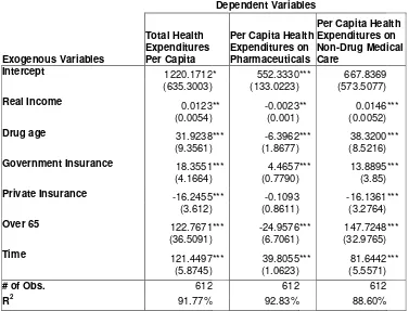
First column of Table 2 reports the estimation results for the effect of drug age on per
capita total health expenditures. The positive and statistically significant coefficient of the
variable “drug age” suggests that the newer the drugs prescribed in a state are, the lower the
total per capita health spending in that state. This implies that newer drugs not only increase
the quality of medical care but also actually lower the total health expenditures. Usually
newer drugs have lower side effects, thus patients would be willing to pay more for them.
Moreover, due to treatment expansion effects, newer drugs would expand the potential patient
19 Levin, Lin, and Chu (2002)
pool. Naturally, as the number of patients to be treated increases, the total treatment costs also
increases. However, similar to the results found in the literature that we have discussed earlier,
our findings imply that the newer medicines are so effective that even if there are more
patients to be treated and each patient is willing to pay more for the lower side effects, the
total spending decreases. However, earlier studies generally use individual and/or event level
data; therefore, they do not consider the treatment expansion effects. Since we use aggregate
state level data, our results are stronger. As an example, a one-year decrease in the average
age of prescribed drugs causes per capita health expenditures to decrease by $31.92. This
amounts to a significant reduction of $171,974,723 for an average state population of
5,387,038 for our sample period.
The estimated coefficients of other exogenous variables are generally inline with the
prior expectations. The positive coefficient on per capita income suggests that on average,
patients of wealthier states spent more on health care because they are willing and able to do
so. In addition, sickness or death is costlier for them than the residents of lower income states
due to working productivity differences. Indeed, the positive relationship between income and
health spending is a common result found in the health expenditure literature.
Interestingly, we find a positive (negative) relationship between the percentage of
government (private) insurance coverage and the HCE. One possible reason is that the cost
containment strategies of private insurance firms are more successful than that of the public
agencies. However, it is also possible that the private insurance companies select the
relatively low cost patients, and government insurance is generally for the poor and old who
have a higher possibility of getting sick and who need more medical care.
The percentage of the population over 65 has a positive relationship with the health
expenditures as expected. The older the state population the more higher the average health
spending. Time trend is also positive and significant. Even after controlling for income,
insurance, demographic effects and the technological improvements in pharmaceuticals, the
health expenditures still rise as time passes. Cost increasing technological improvements on
other areas of medical care could be a reason for that.21 Alternatively, modern life style, which does not require physical activity, encourages unhealthy diet, and causes stress could be the
cause of health problems and higher health care spending.22 Finally, there might be more subtle influences of demographic shifts on health spending that are measured poorly by the
demographic variable that we employ, which is the percentage of population over 65.
In the second column of the Table 2, the health expenditures on pharmaceutical drugs
is the dependent variable. As expected, relatively newer drugs cost more. The negative
coefficient of “drug age” indicates that the states in which relatively newer drugs are
prescribed spent more on pharmaceuticals. This result is parallel to the earlier studies. Newer
drugs are more expensive than older ones. A one-year decrease in the average age of
prescribed drugs causes the per capita health expenditures on pharmaceutical drugs to
increase by $6.4.
On the third column of Table 2, non-drug health expenditures is the dependent
variable. The hypothesis we test in this regression is that the newer drugs save money since
they lower the expenditures on other types of medical services like physician services,
hospital stays, and surgical operations. The positive coefficient of drug age implies that the
data confirm our hypothesis. Higher technology (newer) drugs are more effective than the
relatively older ones, which cause the patients who take them to utilize other types of medical
services less.
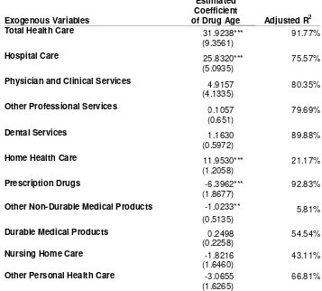
Table 3 reports the estimated coefficient of “drug age” on each HCE category reported
by the Center for Medicare and Medicaid Services, as discussed in Section 4.23 Technological improvements in pharmaceuticals reduce the hospital care and home health
care expenditures the most. Hospital care spending category includes revenues received for all
services provided by hospitals to patients. Home health care includes medical care services
delivered in the home-by-home health agencies.24 Probably physicians are both substitutes and complements for prescription drugs. The results also suggest that spending on other
non-durable medical products is increasing with the newer drugs. The category of other
non-durable medical products includes items such as bandages, surgical and medical instruments
and nonprescription drugs. Negative sign of the coefficient is probably due to mechanical
reasons since drug age variable also includes the age of nonprescription drugs. Similar to
prescription drugs, younger and newer nonprescription drugs are more expensive than the
older ones so as the drug age variable gets bigger the expenditure on nonprescription drugs
declines.
23 We only report and discuss the estimated coefficient of the variable “drug age”. Full regression results are
available from the authors upon request.
Table 4 reports the results from estimating equation 2 that employs first differences of
all variables. In a way, this technique will indicate the short-run effects of newer drugs on
total health spending. The results are similar to the ones from our earlier estimations. Newer
drugs decrease the total health spending. Short run estimations also confirm our hypothesis,
which states that newer drugs are so effective that they lower the demand for other types of
medical care and reduce total health care expenditures. We see similar results when we look
at the short run effects of drug age on various categories of health care expenditures, reported
in Table 5. Newer drugs reduce hospital care and home health care expenditures while
increasing non-durable medical products spending. In addition, newer pharmaceutical
products also lower the expenditure on durable medical products in the short run.
7. Conclusion
In this paper, we studied the influence of the technological improvement in
pharmaceutical technology on health care spending using US State level panel data. We find
that even if newer drugs are more expensive than their predecessors, they are much more
effective so that theyreduce total health expenditures by lowering the need for other types of
medical services.
Earlier studies on the subject have not analyzed the treatment expansion effects, i.e.,
the ability to treat hitherto untreatable patients, of the new drugs. Treatment expansion effects
almost certainly would increase the total health expenditures unlike the treatment substitution
effects. Some of the earlier studies found that newer drugs lower the per patient health
expenditures. However, many new drugs also expand the potential patient pool. Thus in
theory, even if new drugs lower per patient expenditures they could increase the total health
expenditures in a state by treating hitherto untreatable patients. However, our results indicate
that is not the case for US States. By using aggregate data, we show that the newer drugs
lower total health expenditures in a state.
Although most health economists believe that the rising trend in health spending is
partly due to improvement in health technologies, many studies including ours conclude that
the technological improvement in pharmaceutical products does not rise the health spending
but reduces it. This apparent controversy needs an explanation. Many studies have shown that
input use in health production is not efficient everywhere. Fisher et al (2003a, 2003b)
conclude that high spending differences between states are almost entirely due to greater
tests and minor procedures, and greater use of the hospital and intensive care unit. Moreover,
they also conclude that the pattern of practice observed in higher-spending regions does not
result in improved survival, slower decline in functional status, or improved satisfaction with
care. These conclusions imply that high spending regions use wrong types of technologically
advanced medical goods and services, since the government officials play a significant role in
planning of the medical markets.
Our results suggest that regulatory and reimbursement policies toward technologically
better medical goods and services should be reconsidered, and usage of newer drugs should be
encouraged more than usage of newer versions of non-pharmaceutical medical goods and
REFERENCES
Acemoglu D., and Linn J., (2004) “Market Size in Innovation: Theory and Evidence from the
Pharmaceutical Industry”, Quarterly Journal of Economics, August, volume 119, pp.
1049-1090.
Baicker K., and Chandra A., (2004) “Medicare Spending, the Physician Workforce, and Beneficiaries’ Quality of Care”, Health Affairs, April 7, Web Exclusive
Civan A., and Maloney M. (2006) "The Determinants of Pharmaceutical Research and Development Investments," Contributions to Economic Analysis & Policy Vol. 5 : Iss. 1, Article 28.
Cutler D., McClellan M., and Newhouse J., (1998) “What Has Increased Medical-Care
Spending Bought?”The American Economic Review, Vol. 88, No. 2, Papers and Proceedings
pp. 132-136.
Cutler D., and McClellan M., (2001) “Is Technological Change In Medicine Worth It?”
Health Affairs S e p t e m b e r / O c t o b e r
Danzon P., Wang R., and Wang L., (2005) “The Impact of Price Regulation on the Launch
Delay of New Drugs” Health Economics, 14(3)
Duggan M., (2005), “Do New Prescription Drugs Pay For Themselves? The Case Of
Second-Generation Antipsychotics” Journal of Health Economics, 24 pp. 1–31
Duggan M., and Evans W., (2007) “Estimating the Impact of Medical Innovation: A Case Study of HIV Antiretroviral Treatments" mimeo (http://www.econ.umd.edu/~duggan/aids-paper.pdf) accessed on 11-19-2007
Fisher E., Wennberg D., Stukel T., Gottlieb D., Lucas F., and Pinder E., (2003) “The
Implications of Regional Variations in Medicare Spending. Part 1: The Content, Quality, and Accessibility of Care”, Annals of Internal Medicine, Vol: 138(4) pp: 273-287
Fisher E., Wennberg D., Stukel T., Gottlieb D., Lucas F., and Pinder E., (2003) “The Implications of Regional Variations in Medicare Spending. Part 2: Health Outcomes and Satisfaction with Care”, Annals of Internal Medicine, Vol: 138(4) pp: 288-298
Garber A., (2006) “Perspective To Use Technology Better” Health Affairs, 25(2) web exclusive
Gerdtham, U.-G., J. Sdgaard, B. Jnsson and E Andersson (1992), "A Pooled Cross-section Analysis of the Health Expenditure of the OECD countries", in: P. Zweifel and H. Frech, eds., Health Economics Worldwide
Gerdtham, U.G., Lothgren, M., (2000). On stationarity and cointegration of international health expenditure and GDP. Journal of Health Economics 19, 461-475.
Grabowski H.G., Vernon J., and DiMasi J.A., (2002) "Returns on Research and Development for 1990s New Drug Introductions," Pharmacoeconomics, 20(15) Supp. 3, 11-29.
Hudson T., Sullivan G., Feng W.,Owen R., and Thrush C., (2003) “Economic Evaluations of
Novel Antipsychotic Medications: A Literature Review” Schizophrenia Research 60 pp:199–
218
Karlsson, S., and Lothgren M., 2000, “On the Power and Interpretation of Panel Unit Root Tests”, Economics Letters 66, 249-55.
Levin, A., Chien-Fu L., and Chu C.S., 2002, Unit Root Tests in Panel Data: Asymptotic and Finite-Sample Properties, Journal of Econometrics 108, 1-24.
Lichtenberg F., (1996) “Do (More and Better) Drugs Keep People Out of Hospitals?” The
American Economic Review, Vol. 86, No. 2, Papers and Proceedings pp. 384-388.
Lichtenberg F., (2000) “The Benefits And Costs Of Newer Drugs: Evidence From The
1996 Medical Expenditure Panel Survey” CESifo Working Paper Series Working Paper No.
404
Lichtenberg F., (2001)“Are the Benefits of Newer Drugs Worth Their Cost? Evidence from
the 1996 MEPS,” Health Affairs 20(5), September/October 2001, 241-51.
Lichtenberg F., (2002) “Benefits And Costs Of Newer Drugs: An Update” NBER Working Paper 8996
Lichtenberg F., (2006) “The Impact of Increased Utilization of HIV Drugs on Longevity and
Medical Expenditure: An Assessment Based on Aggregate U.S. Time-series Data,” Expert
Review of Pharmacoeconomics and Outcomes Research, Volume 6, Number 4, August, pp. 425-436.
McGinnis, J., Foege, W.H., (1993) ‘Actual Causes of Death in the United States’ Journal of the American Medical Association 270, 2207–2212
Murphy K. M., and Topel R., (2003) “The Economic Value of Medical Research ,” in
Measuring the Gains from Medical Research: An Economic Approach, ed. by Kevin M. Murphy and Robert H. Topel (Chicago: University of Chicago Press, 2003).
National Institute for Health Care Management Research and Educational Foundation
(1999), Factors Affecting the Growth of Prescription Drug Expenditures, Washington.
Newhouse J., (1992) “Medical Care Costs: How Much Welfare Loss?” The Journal of
Economic Perspectives, Vol. 6, No. 3. (Summer), pp. 3-21.
Ng S., and Perron P., 2001, Lag Length Selection and the Construction of Unit Root Tests
with Good Size and Power, Econometrica 69, 1519-54.
Pammolli F., Riccaboni M., Oglialoro C., Magazzini L., Baio G., and Salerno N., (2005) “Medical Devices Competitiveness And Impact On Public Health Expenditure” Center for the Economic Analysis of Competitiveness, Markets and Regulation (CERM), Rome, Italy; prepared for the Directorate Enterprise of the European Commission, accessed on 11-22-2007
http://ec.europa.eu/enterprise/medical_devices/c_f_f/md_final_report.pdf
Slade E., and Anderson G., (2001) “The Relationship Between per Capita Income and Diffusion of Medical Technologies” Health Policy, 58, pp:1-14
Table 1. Summary Statistics ! " # ! # $ % # $ $ ## & & ' ' % $ ( ) * + , , # ,# # , - #
- # &!.
/ #
# . #
& & * # ##
00
# #
! 1
+ 0
2 . 3 & 4 ! $ # ' ! 5 5!
5 * #
6 ## . 1 #
7 , #
$ # ' ! 8 ## 8 3 9 : # : * # #* # : * # & # # . #*
Table 2. Effects of Drug Age on Health Expenditure
This table reports results from estimation of equation 1 by using the fixed effects regression. Heteroskedasticity-robust standard errors are reported in parentheses. ***, ** and * denotes significance levels at the 1%, 5% and 10% levels, respectively.
Dependent Variables
Exogenous Variables
Total Health Expenditures Per Capita
Per Capita Health Expenditures on Pharmaceuticals
Per Capita Health Expenditures on Non-Drug Medical Care
Intercept 1220.1712* 552.3330*** 667.8369
(635.3003) (133.0223) (573.5077)
Real Income 0.0123** -0.0023** 0.0146 ***
(0.0054) (0.001) (0.0052)
Drug age 31.9238*** -6.3962*** 38.3200 ***
(9.3561) (1.8677) (8.5216)
Government Insurance 18.3551*** 4.4657*** 13.8895 ***
(4.1664) (0.7790) (3.85)
Private Insurance -16.2455*** -0.1093 -16.1361 ***
(3.612) (0.8611) (3.2764)
Over 65 122.7671*** -24.9576*** 147.7248 ***
(36.5091) (6.7061) (32.9765)
Time 121.4497*** 39.8055*** 81.6442 ***
(5.8745) (1.0623) (5.5571)
# of Obs. 612 612 612
Table 3. Effects of Drug Age on Various Health Expenditure Categories
This table reports the estimated coefficient of the variable Drug Age for each health care category from estimation of equation 1 by using the fixed effects regression. Heteroskedasticity-robust standard errors are reported in parentheses. ***, ** and * denotes significance levels at the 1%, 5% and 10% levels, respectively.
Exogenous Variables
Estimated Coefficient
of Drug Age Adjusted R2
Total Health Care 31.9238*** 91.77%
(9.3561)
Hospital Care 25.8320*** 75.57%
(5.0935)
Physician and Clinical Services 4.9157 80.35%
(4.1335)
Other Professional Services 0.1057 79.69%
(0.651)
Dental Services 1.1630 89.88%
(0.5972)
Home Health Care 11.9530*** 21.17%
(1.2058)
Prescription Drugs -6.3962*** 92.83%
(1.8677)
Other Non-Durable Medical Products -1.0233** 5.81%
(0.5135)
Durable Medical Products 0.2498 54.54%
(0.2258)
Nursing Home Care -1.8216 43.11%
(1.6460)
Other Personal Health Care -3.0655 66.81%
Table 4. Short Run Effects of Drug Age on Health Expenditure
This table reports results from estimation of equation 2 by using the fixed effects regression. Heteroskedasticity-robust standard errors are reported in parentheses. ***, ** and * denotes significance levels at the 1%, 5% and 10% levels, respectively.
Dependent Variables
Exogenous Variables
(Total Health Expenditures Per Capita)
(Per Capita Health
Expenditures on Pharmaceuticals)
(Per Capita Health Expenditures on Non-Drug Medical Care)
Intercept 122.0779 *** 34.1757 87.9022***
(8.5622 ) (1.0583) (8.0828)
(Real Income) 0.0207 ** -0.0007 0.0214**
(0.0091) (0.0008) (0.0085)
(Drug age) 23.7627 *** -1.0592 24.8219***
(5.5652) (1.0984) (5.1682)
(Government Insurance) 3.0362 0.1489 2.8873
(2.1535) (0.3830) (1.9763)
(Private Insurance) -6.0151 *** -0.5812 -5.4339***
(1.7518) (0.3593) (1.6130)
(Over 65) 308.8451 *** -8.5133*** 317.3583***
(103.6278) (10.0655) (95.5956)
# of Obs. 612 612 612
Table 5. Short run Effects of Drug Age on Various Health Expenditure Categories
This table reports the estimated coefficient of the variable (Drug Age) for each health care category from estimation of equation 2 by using the fixed effects regression. Heteroskedasticity-robust standard errors are reported in parentheses. ***, ** and * denotes significance levels at the 1%, 5% and 10% levels, respectively.
Exogenous Variables
Estimated Coefficient
of (Drug Age) Adjusted R2
(Total Health Care) 23.7627 *** 27.08%
(5.5652)
(Hospital Care) 14.8053 *** 24.74%
(3.3580)
(Physician and Clinical Services) 1.0508 1.63%
(2.8826)
(Other Professional Services) -0.1574 5.98%
(0.5303)
(Dental Services) 1.1927 ** 2.78%
(0.6386)
(Home Health Care) 6.3186 *** 17.48%
(0.8170)
(Prescription Drugs) -1.0592 * 0.87%
(1.0984)
(Other Non-Durable Medical Products) -0.4411 *** 15.75%
(0.2032)
(Durable Medical Products) 0.5777 *** 22.72%
(0.1456)
(Nursing Home Care) 0.2531 7.91%
(1.0056)
(Other Personal Health Care) 1.2366 ** 2.53%
Appendix A. Definitions of Health Care Expenditure Categories Reported by the Center for Medicare and Medicaid Services
Following definitions of the categories of the health care expenditures are extracted from the
links below:
• ••
• 0;<< & * 1< # + =30 # ' < # <0 1> *. 0 %
• ••
• 0;<< & * 1< # + =30 # ' < # < > 0 %
1. Personal Health Care: "Personal health care" is comprised of therapeutic goods or
services rendered to treat or prevent a specific disease or condition in a specific person.
2. Hospital Care: Hospital care spending is defined to cover revenues received for all
services provided by hospitals to patients. Thus, expenditures include revenues received to
cover room and board, ancillary services such as operating room fees, services of resident
physicians, inpatient pharmacy, hospital-based nursing home care, hospital-based home
health care and fees for any other services billed by the hospital.
3. Physician and Clinical Services: The expenditures for physician services are estimated
in three pieces: (1) expenditures in private physician offices and clinics and specialty
clinics that include family planning centers, outpatient mental health and substance abuse
centers, all other outpatient care facilities, and kidney dialysis centers. ; (2) fees of
independently billing laboratories; and (3) clinics operated by the U.S. Department of
Veterans Affairs (DVA) and the U.S. Indian Health Service.
4. Other Professional Services: "Other professional services" covers spending for services
provided by health practitioners other than physicians and dentists. Professional services
include those provided by private-duty nurses, chiropractors, podiatrists, optometrists and
physical, occupational and speech therapists, among others.
5. Dental Services: Expenditures in Offices and Clinics of Dentists (NAICS 6212) are based
on State distributions of business receipts from taxable establishments reported in the
1977, 1982, 1987, 1992, 1997, and 2002 CSI (U.S. Bureau of the Census, 2005).
6. Home Health Care: The home health component of the NHEA measures annual
expenditures for medical care services delivered in the home by freestanding home health
agencies (HHAs). NAICS 6216 defines home health care providers as private sector
establishments primarily engaged in providing skilled nursing services in the home, along
services; physical therapy; medical social services; medications; medical equipment and
supplies; counseling; 24-hour home care; occupation and vocational therapy; dietary and
nutritional services; speech therapy; audiology; and high-tech care, such as intravenous
therapy.
7. Prescription Drugs: The category of prescription drugs includes retail sales of
human-use dosage-form drugs, biologicals and diagnostic products. The transactions to purchase
prescription drugs occur in community pharmacies, grocery store pharmacies, mail-order
establishments, and mass-merchandising establishments.
8. Other Non-Durable Medical Products: The category of other non-durable medical
products includes such items as rubber medical sundries, heating pads, bandages, and
nonprescription drugs and analgesics. Nonprescription drugs sold over the counter include
those marketed to the general public and those promoted to the medical professions and
comprise products such as analgesics, and cough and allergy medications. Finally,
medical sundries primarily include such items as surgical and medical instruments,
surgical dressings, and diagnostic products such as needles and thermometers.
9. Durable Medical Products: Expenditures in this category represent retail sales of items
such as contact lenses, eyeglasses and other ophthalmic products, surgical and orthopedic
products, equipment rental, oxygen and hearing aids. Durable products generally have a
useful life of over three years whereas non-durable products last less than three years.
10.Nursing Home Care: Expenditures reported in this category are for services provided by
freestanding nursing homes. These facilities are defined in the 1997 NAICS as private
sector establishments primarily engaged in providing inpatient nursing and rehabilitative
services and continuous personal care services to persons requiring nursing care (NAICS
6231) and continuing care retirement communities with on-site nursing care facilities
(NAICS 623311).
11.Other Personal Health Care: Privately funded other personal health care consists of
industrial in-plant services provided by employers for the health care needs of their
Appendix B. Unit Root tests
Panel A reports t-statistics from Levin-Lin-Chu unit-root test for the optimal lag lengths of 0, 1, or 2, produced by the method described in Ng and Perron (2001). The null hypothesis is that the variable has a unit root.***,**, and * indicate that unit-root is rejected at the 1%, 5%, and 10% levels, respectively. Panel B reports the % of states for which the variable's stationary is not rejected by a KPSS test in which the null hypothesis is that the variable is stationary.
Panel A. Levin-Lin-Chu test
Lags
Variable 0 1 2
realhcepercap_1 -6.9535*** -5.0735*** -6.3099 *** realhcepercap_2 -7.3137*** -6.8123*** 1.3565 realhcepercap_3 -7.7661*** -5.2772*** -3.0045 *** realhcepercap_4 -6.8513*** -8.0869*** -7.2043 *** realhcepercap_5 -10.5225*** -4.2779*** -1.7984 ** realhcepercap_6 -5.6311*** -8.7841*** -2.3944 *** realhcepercap_7 -1.4149* -2.0435** -7.4251 *** realhcepercap_8 -5.4724*** -8.9696*** -14.6721 *** realhcepercap_9 -6.3982*** -11.7145*** -15.3161 *** realhcepercap_10 -8.5772*** -9.3637*** -7.2259 *** realhcepercap_11 -5.1288*** -12.4175*** -3.6509 *** realhcepercap_1_7 -7.5224*** -5.5610*** -5.6627 *** percaprealinc -3.9461*** -4.2670*** -1.4060 *
Panel B. KPSS test
Variable 5%: 2.5%: 1%: