Using Choice-Based Conjoint Data as Input in ELECTRE
II: University Preference Case in Turkey
Tutku Tuncalı Yaman
Faculty of Economic and Administrative Sciences, Beykent University, Turkey
Copyright©2019 by authors, all rights reserved. Authors agree that this article remains permanently open access under the terms of the Creative Commons Attribution License 4.0 International License
Abstract
The main objective of this study is presenting usage of conjoint data in one of the multi criteria decision techniques (MCDM) ELECTRE II in the context of decision-making process. The approach has been implemented by establishing an objective ranking of private universities in the context of university candidates’ preferences. ELECTRE II procedure is performed on the factors affecting the preference of private universities among candidates and the investment expenditure distribution of the universities. Preference data were collected by Choice-Based Conjoint (CBC) method from 296 students who were in the preference process after 2016 university entrance exams in Turkey. The results obtained from CBC were used as input in ELECTRE II in order to determine a complete and objective ranking of universities. As a result, it could be seen how the rankings differ according to student preferences when investment expenditure areas of universities change the weights of factors. This approach also allowed us to describe the market situation in general thus each university could make a comparative assessment of its own.Keywords
Choice-Based Conjoint Analysis,ELECTRE II, Multiple Criteria Decision Making
1. Introduction
Conjoint analysis (CA) has a widespread usage in determination of consumer preferences with its different approaches after it was developed in early ‘60s [1,2]. A well-known approach in conjoint measurement is called Choice-Based Conjoint (CBC) and it revealed strong acceptance in marketing research after McFadden’s 1986 study [3]. Lately, conjoint scores started to be used as an input for Multi-Dimensional Decision Making (MCDM) methods which run a ranking procedure, such as ELECTRE (Elimination Et (and) Choice Translating Reality) [3]. The technique has six different variations, namely ELECTRE I, ELECTRE II, ELECTRE III, ELECTRE IV, ELECTRE IS and ELECTRE TRI (B-C-nC). ELECTRE II was developed
by scholars Roy and Bertier [4] as a MCDM technique that provides rankings and superiorities of different alternatives according to their attributes’ performance scores. Evaluation method of the technique is based on pairwise comparison of alternatives by concordance & non-discordance principle.
All MCDM techniques have a wide acceptance in decision problems. But in some cases, results could be misleading because of the inaccurate data usage. In general, most of the MCDM techniques evaluate different alternatives according to their importance which is called weights in MCDM terminology, along with their rating/ranking figures. Input data for these assessments are mostly gathered from basic preference, rating a/o ranking questions among alternatives. As the number of questions and alternatives in the questionnaire increases, respondent fatigue may arise. It is a well-known phenomenon that occurs when survey participants become tired of the survey task and the quality of the data they provide begins to deteriorate [5]. One way to avoid this problem is to reduce the total number of alternatives to be evaluated or to change the method of data collection. Conjoint analysis has been seen as the appropriate method for collecting data to be used as input for decision techniques as it is based on making trade-offs between different alternatives as a method of data collection and offers the opportunity to evaluate a large number of alternatives more quickly than basic rating/ranking based questionnaires.
This demonstrative study was conducted under the light of given perspective above. In the following sections of this paper, main objective will be discussed and a brief information about CA, CBC and ELECTRE II will be provided. It will be followed by the results obtained from CBC and ELECTRE II methodologies. The last two sections include discussions and conclusions of the study.
2. Objectives
this purpose, the university preference problem dealt by both public and private university candidates in Turkey, was chosen as a multi criteria decision problem. The main motif upon the selection of this problem is the rising uncertainty in the recent years among students due to the increase in the number of private universities. Turkish educational system, based on the state universities until 2000’s, witnessed a significant rise in the number of private universities, starting from 2010’s. The candidates experience confusion about whether their expectations will be fulfilled by these new universities; for there is not enough experience-based data: All the new universities have just started their admissions. Thus, the preference process of the potential students is solely based on their university exam grades. Within this context, the study first clarified the reasons of students’ preferences along their importance level by using CA; then used the performance comparisons of the newly established universities’ according to these requirements as weights in ELECTRE II and related them to the investment expenditures of these universities.
Detailed information will be provided in the following sections.
3. Materials and Methods
The application of the proposed approach was made within the framework of the investment expenditures of the universities with the factors affecting the preferences of the university candidates.
3.1. Sample
In the context of the purpose, it is important to define targeted population. According to ÖSYM (Student Selection and Placement Center) data, the number of students who attended YGS (Higher Education Entrance Exam) in 2016 and received at least 150 points (minimum score for candidates to make any preference) from any score type was 1.879.812 [6]. This number constitutes the sampling frame of the research with the candidate students. The scope of the study is restricted to private universities located in Istanbul.
Determination of adequate sample size for CA may vary according to the subject of the research and the type of analysis. Akaah and Korgaonkar [7]stated that the sample size was ideal between 100 and 1000, but the observation of 300 and 550 people would be sufficient, while Green and DeSarbo [8] mentioned that they can make effective estimates with smaller samples. In this context, the sample size of the study was determined as 300.
In the sampling process, the private universities in Istanbul, which were considered within the scope of the research objectives, were ranked according to their base scores for university entrance exam and annual tuition fees for the same departments (BA level, departments of administrative sciences). Following the grouping of
universities with similar scores and similar fees for the same departments, 7 of 12 newly established universities – unknown to students- have been randomly selected for sampling. Due to commercial ethics, the names of the selected schools will not be given explicitly within the scope of the study and will be referred to with codes where necessary.
As a result of sampling, two foundation universities (Private universities established by Foundations) were selected for performing the field study. The participants were selected randomly from the candidate students who came to make university choices during the pre-event days of these two universities during the 2016-2017 period.
In addition to collecting preference data via CA, it is planned to collect data from private university administrations in order to determine investment expenditure areas in the aim of being preferable by candidates. This data will be used as attribute weights in the ELECTRE II.
3.2. Data Collection
3.2.1. Pilot Study
The first step for the data collection phase of the research is the validity of the reasons of university preference for candidate students by a pilot study. In October 2015, this pilot study was conducted among first grade freshman students in three private universities in Istanbul. These three schools were found to be equivalent to each other in terms of placement scores and prices. Within the scope of the study, 40 freshmen selected by random sampling were interviewed face-to-face. The questioned reasons for preference in the pilot study are mostly taken from previous researches [9-18]conducted abroad. It is important to assess whether the same reasons are valid in Turkey’s process. In this context, an open-ended “Other” option was also added in questionnaire in order to be able to determine an uncovered/exceptional reason by the pilot study. However, it was observed that there were no “other” reasons other than the factors that were previously determined. Hence the pre-defined factors were accepted as valid factors for university preference which will be included in conjoint design.
3.2.2. Conjoint Study
Software 4.10 CBC System 2.7 Module was used in both data collection and analysis phase. In the program, creation of query cards is completely random, so that each interviewer chose from a differentiated set of cards, and all possible combinations were evaluated. The purpose of the study was explained to the participants at the beginning of the questionnaire, and at the moment (during the university preference stage) they were asked whether they would be able to select the options that were shown on the cards.
In the field study, a total of 310 students have been evaluated by computer assisted face-to-face interviews. 14 Questionnaires have been omitted due to incompleteness and a final data of 296 people was included in the analysis. 3.2.3. Weight Data
The information obtained from the university administrations were provided from public relations managers of ten different private universities via e-mail and phone calls between June and August 2016.
3.3. Data Analysis
The methodology followed in the data analysis can be explained as follows:
1. As a result of the pilot study conducted in October 2015, the most prominent reasons were used as input in the conjoint design. These preference factors were confirmed both by university administrations and expert guidance teachers, on whether they were significantly important in the process of university choice.
2. Conjoint design was established on the reasons of preference (Academic reputation, Campus facilities, Location / Ease of transportation and department diversity) and the names of the preferred universities. The data collection process was completed in July 2016 with the CBC method based on the prepared design.
3. During the sampling period, the public relations managers of 12 universities have been reached by e-mail and telephone and have been asked about the extent of investment expenditures of their
universities on the factors selected within the context of the pilot study and included within the conjoint design (Academic reputation, Campus facilities, Location / Ease of transportation and department diversity). 10 of 12 Universities have provided a response. In order to ease of calculations, the managers were asked to carry out the
evaluations of these properties by weighting them over 100 (sum up to 100).
4. The share of the investments made by universities to be preferred was determined as weights and the utility scores of the students' evaluations which had been obtained from CA were used as inputs in the decision matrix in ELECTRE II. As a result of the
application of the method, a preference ranking was made among the universities.
Conjoint data was analyzed by Sawtooth Software 4.10 CBC System 2.7 package program. Calculations for ELECTRE II were realized with MS Excel 2003.
3.4. Methods
A brief information about the methods used will be discussed under this topic.
3.4.1. Conjoint Analysis
Conjoint Analysis, which is defined as a kind of “Thought Experiment” [19], is basically a technique for measuring how and by what a multi-product choice is made by consumers. Therefore, in today's markets where a wide range of products and services are available, new product development or improvement of existing products is one of the main purposes of conjoint methodology in marketing research.
The technique was developed on the basis of Conjoint Measurement by Luce and Tukey [2]. After the introduction in Green and Srinivasan's [20] study, many computer software such as Sawtooth Software, were developed for conducting the analysis. While most of these programs calculate the importance of product features interacting with each other, they also allow the user to simulate different scenarios. Sawtooth Software differs from the others in the design of data collection process and the display of product cards that will enable participants to evaluate the field survey.
As a general definition, CA is a technique that is used in the measurement of preferences and is based on a decompositional approach. In compositional methods, parameters are determined directly by the decision-maker. On the other hand, in decompositional approaches, these parameters are obtained from the holistic evaluation of the answers of the decision makers (rating, preference, purchasing tendency, i.e.). The statistical process behind the analysis works on calculating the contribution of each attribute and its level to the formation of the profiles. According to Green and Srinivasan [20], the basic steps of applying the analysis are:
1. Determination of attributes and levels, 2. Definition of stimulus (product set),
3. Determination of presentation method of stimulus, 4. Determination of the data collection method and
measurement scale,
5. Selection of model and estimation method, 6. Selection of simulation element.
Decision methods of related steps will be detailed in the next section with their applications.
3.4.1.1. Determination of Attributes and Levels
managers of the product/service. Therefore, those who do not have any relative importance in feature selection are not included in the study [21].
Providing the evaluation of all possible features and levels of related product/service by the participant is called as orthogonal factorial design in conjoint studies [22]. This is the most commonly used approach. If four two-level attributes are to be used, the full factorial design will require a total of 2𝑛𝑛= 24= 16 product profiles to be evaluated. However, in such designs, the number of profiles to be evaluated by the participants can sometimes be far from providing a healthy assessment. Orthogonal Fractional Factorial Design is often used in such cases [20]. This method allows estimation of the utility scores (a.k.a. main effects) of the attributes. On the other hand, these designs can predict more limited (e.g. first level) interactional effects. For instance, if there is a full profile design in which five two-level attributes will be evaluated (32 profiles in total), using a half-replicate design approach can reduce the number of profiles to be evaluated from 32 to 16. In such a design, some of the main and interactive effects can be confused. Although this method is used in some applications, the number of profiles to be evaluated remains high, so some profiles are combined into blocks to form a partially balanced block design. In practice, participants evaluate different blocks of profiles.
3.4.1.2. Definition of Stimulus
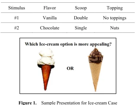
Once the properties and levels of the product have been determined, the product combination to be evaluated is called as stimulus. As an example, given is an ice-cream product with three attributes which are flavor, scoop and topping. Related levels of each attribute are chocolate and vanilla, double and single, no toppings and chocolate chunks respectively. An example stimulus set of mentioned case is illustrated below.
Table 1. Example Stimulus Set for Ice-cream Case
Stimulus Flavor Scoop Topping #1 Vanilla Double No toppings
[image:4.595.63.293.528.705.2]#2 Chocolate Single Nuts
Figure 1. Sample Presentation for Ice-cream Case
3.4.1.3. Determination of Presentation Method for Stimulus After the formation of product profiles, it should be decided how to display these options to the participant.
Conjoint studies generally use the following methods [23]: 1. Verbal identification: A text that describes the
product profile verbally is shown
2. Profile cards: Show product profile cards containing descriptions of each attribute and levels
3. Visual identification: To show the drawing or photograph of the product to be evaluated 4. Computer-aided design: It is possible to show the
product designs that don't exist
5. Physical evaluation: The display of the product itself After the creation of product profiles, the participant should decide how to display these options. Conjoint studies generally use the following methods:
3.4.1.4. Determination of the Data Collection Method and Measurement Scale
Conjoint Techniques differ in terms of types of studies in marketing research. All of the approaches, which can basically be grouped under three headings, have specific advantages and disadvantages. Choosing the appropriate method for the purpose of research is one of the important points to be decided. The approaches mentioned are [21]:
1. Adaptive Conjoint Analysis: The method developed by Sawtooth Software is preferred in the aim of having a user-friendly interface. However, in some cases it is insufficient to give optimal results. The greatest advantage of this method is that the full profile method can be used to implement the application without evaluating all product features simultaneously. However, with this approach, more than six attributes cannot be evaluated effectively at the same time. Yet this method is also effective in estimating price sensitivity.
2. Conjoint Value Analysis: This method can be used to determine the interactions between utility values for each attribute by using a full profile, pairwise comparison or trade-off approaches.
ignored in some product features especially in the studies where the product price is included. When scoring or ranking are performed, these features may not fully demonstrate their importance. Another advantage of this method is that the calculations are relatively short and easy.
Due to the complexity of the conjoint studies, the most appropriate way to collect data is face-to-face interviews. In this regard, data collection by phone or mail is not preferred due to the possibility of making the product profiles difficult to understand. On the other hand, performing computer-assisted interviews, rather than pen-and-paper alternative, is better especially for adaptive and choice-based conjoint methods [24]. The other data collection methods are detailed as follows:
1. Full-profile Approach: The respondents evaluate all the profiles consisting of combinations of all properties respectively.
2. Trade-off Approach: The respondents evaluate combinations of all levels of the two properties. 3. Paired Comparison Approach: Participants evaluate
profile pairs that include combinations of all features. 4. Experimental Choice Approach: Participants select
one of the profile sets where each profile is determined by all properties
In both the full profile and trade-off approach, evaluation can be based on ranking or scoring. Scores are usually made on an evenly spaced scale of 7 or 9. The paired comparison approach is used in the Adaptive Conjoint Analysis method. 3.4.1.4. Selection Model and Estimation Method
There are four basic models describing the functions that express the multiple attribute preferences of consumers in the context of Conjoint. These are vector model, ideal point model, part-worth model and mixed model. The mathematical representation of these four models is as follows:
1. Vector Model: 𝑦𝑦𝑛𝑛𝑛𝑛=𝑐𝑐𝑛𝑛+∑𝑛𝑛𝑛𝑛=1𝛽𝛽𝑛𝑛𝑛𝑛𝑥𝑥𝑛𝑛𝑛𝑛 (1)
2. Ideal Point: 𝑦𝑦𝑛𝑛𝑛𝑛 =𝑐𝑐𝑛𝑛+∑𝑛𝑛𝑛𝑛=1𝛽𝛽𝑛𝑛𝑛𝑛(𝑥𝑥𝑛𝑛𝑛𝑛− 𝑎𝑎𝑛𝑛𝑛𝑛)2 (2)
3. Part-worth: 𝑦𝑦𝑛𝑛𝑛𝑛=∑𝑛𝑛=1𝑛𝑛 ∑ 𝛽𝛽𝑙𝑙=1𝐿𝐿𝑝𝑝 𝑙𝑙𝑛𝑛𝑓𝑓1(𝑥𝑥𝑛𝑛𝑛𝑛) (3)
4. Mixed Model: The combination of the above three models
Notations:
𝑙= 1, 2, … ,𝑙𝑛𝑛 : Levels of attribute p 𝑥𝑥𝑛𝑛𝑛𝑛: Levels of attribute p at profile k
𝑦𝑦𝑛𝑛𝑛𝑛: Evaluation of nth respondent for profile k 𝑎𝑎𝑛𝑛𝑛𝑛: Ideal point of nth respondent for attribute p
𝑓𝑓1(𝑥𝑥𝑛𝑛𝑛𝑛): Indicator function for first level of attribute p at profile k
Many different methods have been used to evaluate the conjoint data. The selection of the appropriate method is based on the scale that the participant uses in his / her preference assessment for product profiles. The three basic
scales used in the conjoint are: metric / ratio, ranking and nominal (selection based) scales. Metric data is generally used for prediction with ordinary least squares and its significance levels are obtained from here. The most commonly used methods for measurement based on order MONANOVA [25] and LINMAP [26]. Another alternative is the PROBIT model and does not require the assumptions of the LOGIT [27]. However, in the estimation of this model, when the set subject to the selection contains more than three alternatives, it may be problematic that the numerical solution of the fourth and higher dimensional integrals cannot be made. In such cases, McFadden [28] proposed the use of simulation methods for integral calculation.
Sawtooth Software, R and SPSS are easy-to-use programs to estimate the results. For selection-based, adaptive and value-analysis approaches Sawtooth simulation model provides more detailed results than SPSS [29].
However, in conjoint studies, it is very important to collect the data correctly and accurately before the analysis. Although design can be done with many statistical analysis programs such as SPSS Conjoint, R’s optfederov () function in AlgDesign package. Sawtooth Software provides a great advantage with its interface defined in the process. Otherwise, these product cards to be evaluated should be prepared one by one by evaluating each participant with the appropriate combinations.
3.4.2. ELECTRE
The technique was proposed by Roy [30] in 1968 by introducing different techniques with the work of Roy, Bouyssou and Yu, Roy and Bertier [4, 31, 32]. ELECTRE has six different approaches which are called ELECTRE I, ELECTRE II, ELECTRE III, ELECTRE IV, ELECTRE IS, and ELECTRE Tri. All these versions are based on the same fundamental concepts but they differ on some operations and on the type of the decision problem. Specifically, ELECTRE I is used for selecting the problems, ELECTRE TRI for the assignment of those problems and ELECTRE II, III and IV for ranking of the problems [33].
ELECTRE compares all possible pairs of different alternatives on the basis of criteria and takes decisions based on criterion-based scores (Hwang and Yoon, 1981). In binary comparisons, alternatives are chosen by selecting superior performance alternatives. In the process of the method, a decision (pay-off) matrix is created where the performance of all the criteria is shown at the level of available alternatives. The lines in the matrix show alternatives, columns indicate the criteria, the matrix elements indicate the performance of the benchmark alternative in the corresponding row and column.
𝐴=�𝑎𝑎11⋮ ⋯ 𝑎𝑎⋱ 1𝑛𝑛⋮
𝑎𝑎𝑚1 ⋯ 𝑎𝑎𝑚𝑛𝑛
� (4)
elements of the normalized decision matrix are calculated as follows.
𝑟𝑖𝑗= 𝑎𝑖𝑗
�∑𝑚𝑘=1𝑎𝑘𝑗2 (5) In next step, the normalized decision matrix is multiplied by the benchmark weights (0≤ 𝑤𝑛𝑛≤1;∑𝑛𝑛𝑗=1𝑤𝑗) obtained as a priori information to obtain the weighted decision matrix (V), shown below.
𝑉=�𝑟11⋮𝑤1 ⋯ 𝑟⋱ 1𝑛𝑛⋮𝑤𝑛𝑛 𝑟𝑚1𝑤1 ⋯ 𝑎𝑎𝑚𝑛𝑛𝑤𝑛𝑛
� (6)
𝑚(𝑚 −1) number of concordance sets are created for each alternative pair using the weighted decision matrix (V) to determine concordance and discordance matrix. Here, the number of elements must be equal to the number of criteria. Concordance sets (for instance, Alternative #1 and Alternative #2) can be shown as follows:
𝐶=�𝑗�𝑣1𝑗≥ 𝑣2𝑗� (7)
The formula is basically based on comparing row elements with each other in sequence. For instance, when comparing Alternative #1 and Alternative #2, the value of the Alternative #1 for the criteria in third and fourth columns will be equal to or greater than that of the Alternative #2. If it is smaller for other columns, the value will be𝐶12= {3,4}.
Discordance sets are also mutually generated on each set of concordance. The path to be followed in the creation of the discordance matrix is likewise based on the comparison of the line elements. Again, for Alternative #1 and Alternative #2, a set of discordance can be created as follows:
𝐷12=�𝑗�𝑣1𝑗 <𝑣2𝑗� (8)
Discordance set against 𝐶12 in the example above (for a four criterion example) will be 𝐷12= {1,2}. The concordance matrix C and the discordance matrix D are generated using concordance and discordance sets. The approach to constructing (𝑚×𝑚) dimensional compatibility matrix will be used to determine the relative weights for the criteria where the alternatives are superior (or equal). The elements of the concordance matrix that do not value for the diagonal elements are created as follows:
𝐶𝑛𝑛𝑙𝑙=∑𝑗∈𝐶𝑘𝑙𝑤𝑗 (9)
If 𝐶12= {3,4}, according to the above example, the value of the element 𝑐𝑐12 of matrix C will be calculated as 𝐶12=𝑤1+𝑤2. Elements of the discordance matrix are obtained using the following formulation:
𝐷𝑛𝑛𝑙𝑙=
�𝑣𝑘𝑗−𝑣𝑙𝑗� 𝑗∈𝐷𝑘𝑙
𝑚𝑎𝑥
�𝑣𝑘𝑗−𝑣𝑙𝑗� 𝑗
𝑚𝑎𝑥 (10)
In the formulae, numerator shows the maximum difference on discordance index and denominator shows the maximum difference on any creation. The D matrix is also
(𝑚×𝑚)dimensional like C and does not take any value for its diagonal elements.
In the next step towards determining the dominant
criterion, concordance and discordance indexes are made to calculate the matrices of superiority. The concordance index for a pair of alternatives #1 and #2, measures the strength of the hypothesis that alternative #1 is at least as good as alternative #2. The discordance index measures the strength of evidence against this hypothesis. Final ranking of alternatives is obtained from the superiorities according to these indexes.
The concordance superiority matrix (F) is (𝑚×
𝑚) dimensional in size and is found by comparing the alignment matrix elements with the concordance threshold values. If the concordance matrix element is equal to or greater than the threshold value, the element of the concordance superiority matrix takes 1, otherwise takes 0.
𝑐𝑐𝑛𝑛𝑙𝑙≥ 𝑐𝑐̅ → 𝑓𝑓𝑛𝑛𝑙𝑙= 1 (11) 𝑐𝑐𝑛𝑛𝑙𝑙<𝑐𝑐̅ → 𝑓𝑓𝑛𝑛𝑙𝑙= 0 (12) The matrix elements take only 1 and 0 values. The following formula is used to calculate threshold values:
𝑐𝑐̅=𝑚(𝑚−11 )∑𝑚𝑛𝑛=1∑𝑚𝑙𝑙=1𝑐𝑐𝑛𝑛𝑙𝑙 (13) Discordance superiority matrix (G) elements are similarly calculated by comparing discordance matrix elements with the threshold value of discordance. If the discordance matrix element is equal to or greater than the threshold value, the element of the discordance superiority matrix takes 1, otherwise takes 0.
𝑑𝑛𝑛𝑙𝑙≤ 𝑑̅ → 𝑔𝑛𝑛𝑙𝑙= 1 (14)
𝑑𝑛𝑛𝑙𝑙>𝑑̅ → 𝑔𝑛𝑛𝑙𝑙= 0 (15) The elements of the (𝑚×𝑚)dimensional discordance superiority matrix can also take only 1 and 0 values. Calculation of the threshold values is similar to the other and uses the following formula:
𝑑̅=𝑚(𝑚−11 )∑𝑚𝑛𝑛=1∑𝑚𝑙𝑙=1𝑑𝑛𝑛𝑙𝑙 (16) In ELECTRE II, it was necessary to increase threshold values from the average concordance and discordance threshold values in order to evaluate different situations [34].
The total superiority matrix (E) to be used in decision-making is obtained by comparing the elements of concordance superiority and discordance superiority matrix in order to evaluate outranking relations. The lines and columns of the E matrix represent alternatives, and the elements with 1 in both matrices are represented as 1 in E matrix, and 0 in any of them. Hence, it is decided by comparing superior alternatives.
Two elements are used to establish the outranking relationship value for ELECTRE II which are strong
0≤ 𝑝𝑝−≤ 𝑝𝑝0≤ 𝑝𝑝∗≤1
Plus, 𝑞∗,𝑞0 are represented by two degressive discordance levels, and meet the following conditions:
0 <𝑞∗<𝑞0< 1
Posterior to identify concordance and discordance levels, it is possible to establish value for the 𝑅𝑆 and, 𝑅𝑊, calculate strong (𝑉′) and weak (𝑉′′) ranking values, and finally, determine the average ranking 𝑉� for final ranking result [35].
4. Results
In this chapter, the findings of the pilot study, the results of the conjoint analysis which was based on the preferences of the university candidates and ELECTRE II integration practice realized with conjoint measurement data are represented.
4.1. Pilot Study
In the face-to-face pilot survey study, which was attended by 40 freshmen, the reasons of university preference in the literature were offered to the students for their evaluation.
[image:7.595.324.515.80.224.2]Students were asked to mark the factors they considered important in university preferences, and then they were asked to rank 1 to 3 by selecting the three factors they considered the most important. According to the pilot study, the factors that are important in the university preference of the students are as follows:
Table 2. Important Factors in University Preference
Factors %
Presence of the desired field 63 Location / Ease of transportation 55
University 54
Academic reputation of the university 50
Campus facilities 33
4.2. Conjoint Study
According to the results obtained from the pilot study, the following five factors with 16 levels in total, will be included in stimuli to be prepared for the evaluation of candidate students within the scope of conjoint design:
University University A University B University C University D University E University F University G
Academic reputation
Experienced faculty members Inexperienced faculty members Campus facilities
Has an attractive campus Campus facilities are poor Location / Ease of transportation
It is difficult to get to & away from home Easy to get to & away from home Close to home & easy to reach Presence of the desired field
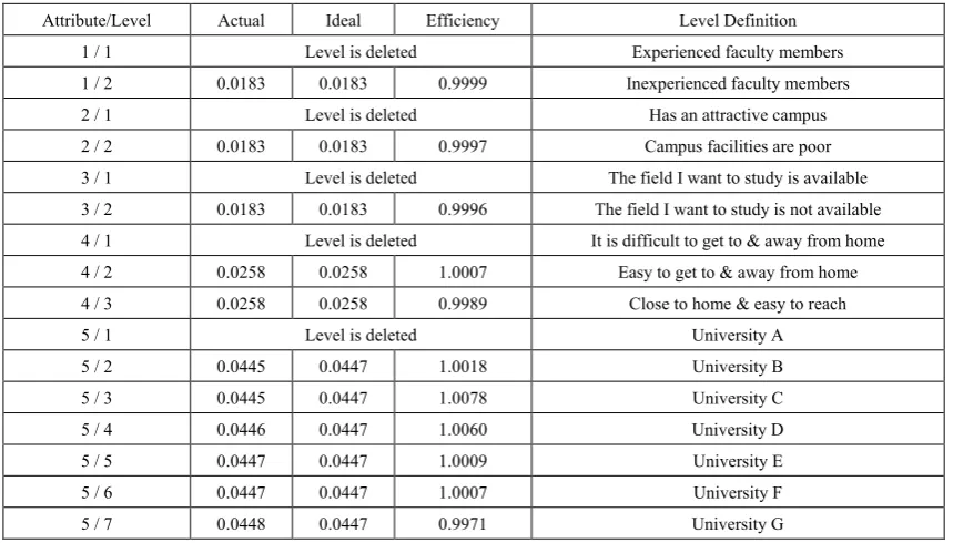
The field I want to study is available The field I want to study is not available 4.2.1. Design Efficiency
Table 3. Design Efficiency
Attribute/Level Actual Ideal Efficiency Level Definition
1 / 1 Level is deleted Experienced faculty members
1 / 2 0.0183 0.0183 0.9999 Inexperienced faculty members
2 / 1 Level is deleted Has an attractive campus
2 / 2 0.0183 0.0183 0.9997 Campus facilities are poor 3 / 1 Level is deleted The field I want to study is available 3 / 2 0.0183 0.0183 0.9996 The field I want to study is not available 4 / 1 Level is deleted It is difficult to get to & away from home 4 / 2 0.0258 0.0258 1.0007 Easy to get to & away from home 4 / 3 0.0258 0.0258 0.9989 Close to home & easy to reach
5 / 1 Level is deleted University A
5 / 2 0.0445 0.0447 1.0018 University B
5 / 3 0.0445 0.0447 1.0078 University C
5 / 4 0.0446 0.0447 1.0060 University D
5 / 5 0.0447 0.0447 1.0009 University E
5 / 6 0.0447 0.0447 1.0007 University F
5 / 7 0.0448 0.0447 0.9971 University G
4.2.2. Model Estimation
Model and utility coefficients at the level of main effects were estimated by Multinomial Logistic Regression (Multinomial LOGIT). Before the interpretation of the coefficients, it is necessary to look at the overall compatibility of the model and the effectiveness of the predictive power. Goodness of fit value (−2𝑙𝑜𝑔𝜆) for ideal model estimated as 4103,43. This value was found as 2578,63 for the main model. Test statistics calculated to test the goodness of fit under the hypothesis of the ideal model is Δ𝐺2= (−2𝑙𝑜𝑔𝜆)
𝑖𝑑𝑒𝑎𝑙𝑙−(−2𝑙𝑜𝑔𝜆)𝑚𝑎𝑖𝑛𝑛= 1524.79with 𝑑𝑓𝑓= 16−5 = 11 (degree of freedom= Number of levels - number of attributes). Table value for test statistic is 𝜒𝜒02,05;11= 19.675. Since the test statistic value is greater than the table critical value, the null hypothesis is rejected. The model created is sufficient for estimation. (Wilks,1938) Other criteria used in favorable model selection are stated below:
Consistent Akaike Info Criterion (CAIC): 5263.82 Percent Certainty:37.15899
Chi Square: 3049.58 Relative Chi Square: 277.23
In the evaluation of the predictive power and adequacy of the model, it is accepted that larger values are better for criteria calculated above. Therefore, predicted model was also found effective [37]. The results obtained from Multinomial LOGIT Model were analyzed by the levels of each factor. Detailed results of estimation are shown in Table 4 below. According to results:
Importance degree of “Experienced faculty members” level for “Academic reputation” attribute interpreted as 0.51143. This coefficient is statistically significant (𝑡𝑡= 25.5,𝑝𝑝< 0.05).
Universities that are considered equivalent in the University factor are shown. Among these, University A was found to have the highest level of importance (effect: 0.31059) (𝑡𝑡= 5.56,𝑝𝑝< 0.05).This value is positive and statistically significant.
When the “Presence of the desired field” attribute is taken into consideration, it is seen that “The field I want to study is available” level has the highest importance for candidate students (effect: 0.7972) and the coefficient of utility in the model is statistically significant (𝑡𝑡= 38.23,𝑝𝑝< 0.05). The opposite level of the same attribute has the same but negative significant value.
Among the levels in the “Location / Ease of transportation” attribute, the “Easy to get to & away from home” level has the highest utility. (effect: 0.11018) (𝑡𝑡= 3.63,𝑝𝑝< 0.05). Another remarkable point here is that the reverse effect of “It is difficult to get to & away from home” level is quite high. (effect: -0.1955) (𝑡𝑡=−6.83,𝑝𝑝< 0.05). The third level in this attribute is; “Close to home & easy to reach” has almost the same degree of significance as the “Easy to get to & away from home” level and the coefficient is statistically significant (effect: 0.0936) (𝑡𝑡= 3.3,𝑝𝑝< 0.05).
Table 4. Multinomial Logistic Regression Estimation Results
Attribute/Level Level Definition Effect Standard Error t 1 / 1 Experienced faculty members 0.51143 0.02006 25.50097 1 / 2 Inexperienced faculty members -0.51143 0.02006 -25.50097 2 / 1 Has an attractive campus 0.32961 0.01816 18.1538 2 / 2 Campus facilities are poor -0.32961 0.01816 -18.1538 3 / 1 The field I want to study is available 0.79723 0.02085 38.2385 3 / 2 The field I want to study is not available -0.79723 0.02085 -38.2385 4 / 1 It is difficult to get to & away from home -0.19550 0.02860 -6.83678 4 / 2 Easy to get to & away from home 0.10182 0.02825 3.60390 4 / 3 Close to home & easy to reach 0.09368 0.02834 3.30514
5 / 1 University A 0.31059 0.05583 5.56317
5 / 2 University B -0.06751 0.05566 -1.21288
5 / 3 University C -0.02838 0.05620 -0.50506
5 / 4 University D -0.10570 0.05485 -1.92732
5 / 5 University E 0.01583 0.05562 0.28453
5 / 6 University F -0.15504 0.05577 -2.77996
5 / 7 University G 0.03023 0.05581 0.54162
4.2.3. Main Effects
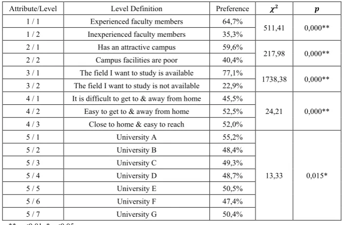
As a result of the analysis made for the main effects, it was observed that “The field I want to study is available” was more preferred than “The field I want to study is not available” in 77% of the cases in “Presence of the desired field” attribute (𝜒𝜒2= 1738.38,𝑝𝑝< 0.01). In the “University” attribute, it was found that A University was preferred more than the other school options with a preference of 55% (𝜒𝜒2= 13.33,𝑝𝑝< 0.05). Among the levels of “Academic reputation”, the “Experienced faculty members” is the most preferred level with 65% (𝜒𝜒2= 511.42,𝑝𝑝< 0.01). The most preferred level for “Campus Facilities” attribute is “Has an attractive campus” with 60% preference percentage (𝜒𝜒2= 217.99,𝑝𝑝<
[image:9.595.130.482.492.726.2]0.01). Among the levels in the “Location / Ease of transportation” attribute, “Easy to get to & away from home” level is the most preferred one with 53% (𝜒𝜒2= 24.21,𝑝𝑝< 0.01). The percentages of preference for each factor are given in the Table 5 below.
Table 5. Preference Percentages for Main Effects
Attribute/Level Level Definition Preference 𝝌𝟐 𝒑
1 / 1 Experienced faculty members 64,7%
511,41 0,000** 1 / 2 Inexperienced faculty members 35,3%
2 / 1 Has an attractive campus 59,6%
217,98 0,000** 2 / 2 Campus facilities are poor 40,4%
3 / 1 The field I want to study is available 77,1%
1738,38 0,000** 3 / 2 The field I want to study is not available 22,9%
4 / 1 It is difficult to get to & away from home 45,5%
24,21 0,000** 4 / 2 Easy to get to & away from home 52,5%
4 / 3 Close to home & easy to reach 52,0%
5 / 1 University A 55,2%
13,33 0,015*
5 / 2 University B 48,4%
5 / 3 University C 49,3%
5 / 4 University D 48,7%
5 / 5 University E 50,5%
5 / 6 University F 47,4%
5 / 7 University G 50,4%
**: p<0.01, *:p<0,05
[image:9.595.128.483.493.725.2]4.3. Determining the Weights of Universities’ Marketing Activities
In order to be used as weights in ELECTRE II procedure, the properties that universities invested in have been determined from the official personnel interviewed in the selected schools (public relations authority or general secretary). During the interviews, the distribution of investments in order to increase the level of preference has been asked to the related personnel. These distribution fields, as stated before, have been gathered from the factors that students placed an emphasis on during their preference period. In the aim of presenting the university’s point of view, the name of the university was categorized under “Brand Awareness”, while the “Presence of the desired field” was categorized under “Department Diversity”. The rest was recorded as per se.
In this context, they were asked to distribute the total 100 points given to the five factors presented to them in a way that represents the relative and individual importance level. Correspondingly, the evaluations made by the school authorities are given in Table 6 below.
According to this, it is evident that the school administrations have invested most in increasing their academic reputation by hiring qualified faculty members, and this factor is followed by investing on brand awareness activities for their schools. The least invested factor is the location of the school and the ease of transportation to school.
Proportional distribution of investments for each factor in a 100-sum scale was organized and the arithmetic mean of attribute based data was accepted as the weighting vector in ELECTRE II.
[image:10.595.125.471.325.487.2]In the following chapter, ELECTRE II application results are detailed and corresponding findings are evaluated in the context of university preference problem.
Table 6. Distributions of Universities’ Investments
University awareness Brand Academic reputation facilities Campus Location Department diversity
A 20 20 20 20 20
B 40 30 10 10 10
C 20 30 15 15 20
D 20 40 20 10 10
E 30 30 15 10 15
F 25 25 20 15 15
G 20 40 20 5 15
H 12 13 25 25 25
J 15 30 15 20 20
K 35 20 15 10 20
Average 23.7 27.8 17.5 14 17
4.4. ELECTRE II
This section depicts the application steps of ELECTRE II method separately. The results of the calculations explained in the Methodology Section in detail are exhibited in matrixes; while their explanations are placed in-between the tables from 7 to 11.
Initial decision (pay-off) matrix (A) of ELECTRE is constituted from conjoint measurement results showed in Table 5. In this matrix where cell values are the performance value of the alternative on related criterion showed below:
Table 7. Initial Decision Matrix
University Location Presence of the desired field facilities Campus reputation Academic
A 0.59 0.80 0.65 0.70
B 0.52 0.76 0.58 0.63
C 0.51 0.79 0.59 0.65
D 0.48 0.75 0.59 0.62
E 0.54 0.77 0.59 0.65
F 0.48 0.74 0.59 0.62
G 0.51 0.79 0.58 0.66
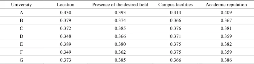
[image:10.595.127.469.600.717.2]Table 8. Normalized Decision Matrix
University Location Presence of the desired field Campus facilities Academic reputation
A 0.430 0.393 0.414 0.409
B 0.379 0.374 0.366 0.367
C 0.372 0.385 0.376 0.381
D 0.348 0.366 0.371 0.359
E 0.389 0.380 0.375 0.382
F 0.349 0.362 0.375 0.359
G 0.373 0.385 0.366 0.386
[image:11.595.85.507.284.421.2]Weighted decision matrix (V) is calculated as multiplying the normalized decision matrix with the weight vector. The investments that the universities provided for the preference factors are used as weight values in this part. The distribution of these investment expenditures were already gathered from the school administrations by the division of 100 points according to the weight of the factors. Here, weight values are indexed to 1 for ease of calculation. These indexed values constitute the Indexed Weight Vector showed below.
Table 9. Weighted Decision Matrix
University Location Presence of the desired field Campus facilities Academic reputation
A 0.079 0.088 0.095 0.149
B 0.070 0.083 0.084 0.134
C 0.068 0.086 0.086 0.139
D 0.064 0.081 0.085 0.131
E 0.071 0.085 0.086 0.139
F 0.064 0.081 0.086 0.131
G 0.068 0.086 0.084 0.141
Weight Vector 14 17 17.5 27.8
Indexed weight vector 0.183 0.223 0.229 0.364
The concordance index measures a weighted number of attributes for which alternative x is preferred or equal to alternative y. In this study these alternatives indicate the evaluated universities. Concordance values were calculated by using Equation (7) and presented in Table 10 below.
Table 10. Concordance Matrix
A B C D E F G
A - 0 0 0 0.00 0.00 0.00
B 1 - 0.81 0.22 1.00 0.22 0.51
C 1 0.18 - 0 0.55 0.00 0.44
D 1 0.77 1 - 1.00 0.41 0.56
E 1 0.00 0.45 0 - 0 0.37
F 1 0.77 1.00 0.58 1 - 1
G 1 0.18 0.23 0.23 0.41 0.23 -
[image:11.595.156.440.654.759.2]The discordance index. measures the strength of the greatest discontent or disagreement among all attributes. When alternative x is selected over alternative y. In other words, it indicates the level of discontent that is accepted when attribute x is selected instead of attribute y. Calculation steps of discordance values were described in Equation (11) before and results presented in Table 11 below.
Table 11. Discordance Matrix
A B C D E F G
A - 0.10 0.07 0.12 0.07 0.12 0.07
B 0.11 - 0.04 0.04 0.04 0.04 0.05
C 0.08 0.04 - 0.06 0.02 0.06 0.02
D 0.14 0.04 0.06 - 0.06 0.01 0.07
E 0.07 0.04 0.02 0.06 - 0.06 0.02
F 0.14 0.04 0.06 0.01 0.06 - 0.08
After computing the concordance and discordance indices for each pair of alternatives, two types of outranking relations are built by comparing these indices with two pairs of threshold values which are: 𝐶∗, 𝐷∗,𝐶−, 𝐷−. 𝐶∗, indicates the average value of 𝐶(𝑥𝑥,𝑦𝑦). 𝐷∗, indicates the average value of 𝐷(𝑥𝑥,𝑦𝑦). 𝐶− and 𝐷− are defined by decision maker accordingly, 𝐶∗>𝐶−, and 𝐷∗<𝐷−. In the final interpretation phase of outranking relations two main rule applied [35].
Rule #1: If 𝐶(𝑥𝑥,𝑦𝑦)≥ 𝐶∗,𝐷(𝑥𝑥,𝑦𝑦)≤ 𝐷∗ and 𝐶(𝑥𝑥,𝑦𝑦)≥ 𝐶(𝑦𝑦,𝑥𝑥) then alternative x is regarded as strongly (S) outranking alternative y.
Rule #2: If 𝐶(𝑥𝑥,𝑦𝑦)≥ 𝐶−,𝐷(𝑥𝑥,𝑦𝑦)≤ 𝐷− and 𝐶(𝑥𝑥,𝑦𝑦)≥ 𝐶(𝑦𝑦,𝑥𝑥) then alternative x is regarded as weakly (W) outranking alternative y.
By using the values of 𝐶∗= 0.34, 𝐷∗= 0.04,𝐶−=
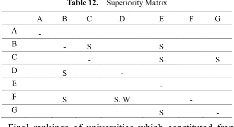
[image:12.595.59.289.307.432.2]0.3, 𝐷−= 0.01, the total superiority matrix constituted and showed below in Table 12.
Table 12. Superiority Matrix
A B C D E F G
A -
B - S S
C - S S
D S -
E -
F S S. W -
G S -
Final rankings of universities which constituted from superiority matrix, could be presented as:
𝐹=𝐴>𝐶=𝐷=𝐺>𝐵>𝐸
5. Conclusions and Discussion
ELECTRE II is a MCDM technique that provides rankings according to superiorities of different alternatives based on to their attributes’ performance scores. Evaluation method of the technique is based on pairwise comparison of alternatives by concordance & discordance principle. However, use of ELECTRE, as well as most MCDM techniques, needs weight values, which are mostly determined subjectively by the decision maker in application. The context of analysis includes the evaluation of various alternatives uniquely within themselves based on different factors rather than a comparison between these various alternatives. The data obtained from this single dimensional evaluation affects the practicality of the results. In order to eliminate this negative tendency and deriving more objective indicators, CA was used to gather alternative based evaluation data. This approach was applied by Zardari, Cordery and Sharma [34] to determine priority in water allocations by using standard conjoint design. But in this study, an eminent approach in conjoint measurement, Choice-Based
Conjoint was adopted to gather preference data.
As an application of the proposed approach, the university preference problem for candidates in Turkey, was chosen as a multi criteria decision problem. The main reason for this selection lies on the fact that state universities have been ruled by Turkey’s higher education system for years. Recently, the number of private universities arose and they started to take role in university candidates’ selection paradigm. However, as sufficient information cannot be gathered about these schools recently included in the system, there appears a significant uncertainty during the preference process. Although the university candidates make their preferences on the assumption that their requirements will be met by these newly established schools, as stated before, there is no concrete evidence that these institutions will fulfill such factors, given that they have not graduated any students yet.
In this context, it is necessary to obtain an objective ranking among these private universities by considering important factors according to the candidates’ university selection process. Thus, interpreting the preference scores of the candidates based solely on CA would not be sufficient. The schools’ performances based on the selected factors by the students would also be critical in the objective ranking.
As a result of the study, realized by empirical data, it could be seen how the rankings differ according to university candidate preferences when investment decision according to different areas of universities change the weights of attributes defined as preference reasons. In addition to that, this approach also allowed to describe the market situation in general thus each university could make a comparative assessment of its own.
Another advantage of the offered approach is that, given the input data in the ELECTRE method, it provides a more objective evaluation within the nature of the problem compared to the subjective evaluation of the decision maker. In numerous ELECTRE implications, the weights are specified by a specific decision maker or a limited number of experts on the subject. Yet, the data about the performances of different alternatives within the analysis is obtained by the singular evaluation of each participant. Thus, the approach of this study has increased the quality and coherence of the data.
Future studies may use the CA data with different MCDM methods, as well as implicate the same approach on the decision making problems in wider and/or different fields.
REFERENCES
[1] K. Govindan, M. B. Jepsen. ELECTRE: A comprehensive literature review on methodologies and applications, European Journal of Operational Research, No.250, 1-29, 2016.
[2] N. Luce, N. Tukey, N. Simultaneous conjoint measurement: A new type of fundamental measurement, Journal of Mathematical Psychology, No.1, 1-27, 1964.
[3] D. McFadden. Estimating household value of electric service reliability with market research data, Marketing Science, Vol.5, No.4, 275-297, 1986.
[4] B. Roy, P. Bertier. La méthode ELECTRE II: Une méthode de classement en présence de critères multiples, Paris, Sema (Metra-International) Direction Scientifique, No.25, 1971. [5] P. Ben-Nun. Respondent fatigue, In Encyclopedia of Survey
Research Methods, Edited by Paul J. Lavrakas, Sage Publications, Inc., 2011.
[6] I. Akbas. Comparison between undergraduate placement examination (LYS) in Turkey and Edexcel International Advanced Levels Examination (IAL) in the world, Green University Review of Social Sciences, Vol. 2, 71-93, 2016. [7] I. P. Akaah, P. K. Korgaonkar. A conjoint investigation of the relative importance of risk relievers in direct marketing, Journal of Advertising Research, Vol.28, 38-44, 1988. [8] P. Green, W. S. DeSarbo. Additive decomposition of
perceptions data via conjoint analysis, Journal of Consumer Research, Vol.5, No.1, 58–65, 1978.
[9] R. F. Krampf, A. C. Heinlein, A. C. Developing marketing strategies and tactics in higher education through target market research, Decision Sciences, No.12, 175-192, 1981. [10]D. W. Chapman. A model of student college choice, The
Journal of Higher Education, Vol.52, No.5, 490-505, 1981. [11]G. J. Hooley, J. E. Lynch. Modelling the student university
choice process through the use of conjoint measurement techniques, European Research, Vol.9, No..4, 158, 1981. [12]R. E. Kallio. Factors influencing the college choice decisions
of graduate students, Research in Higher Education, Vol.36, No.1, 109-124, 1995.
[13]G. N. Soutar, J. P. Turner. Students preferences for university: A conjoint analysis, International Journal of Educational Management, Vol.16, No.1, 40-45, 2002. [14]M. Joseph, B. Joseph. Indonesian students’ perceptions of
choice criteria in the selection of a tertiary ınstitution:
strategic implications, The International Journal of Educational Management, Vol.14, No.1, 40-44, 2000. [15]J. E. Hoyt, A. B. Brown. Identifying college choice factors to
successfully market your institution, College and University, Vol.78, No.4, 3-10, 2003.
[16]C. Veloutsou, J. W. Lewis, R. A. Pton. Consultation and reliability of information sources pertaining to university selection: Some questions answered?, International Journal of Educational Management, Vol.19, No.4, 279- 291, 2005. [17]G. T. Yamamoto. University evaluation-selection: A
Turkish case. International Journal of Educational Management, Vol.20, No.7, 559-569, 2006.
[18]S. Domino, T. Libraire, D. Lutwiller, S. Superczynski. Higher education marketing concerns: factors influence students’ choice of colleges, The Business Review, Vol.6, No.2, 101-111, 2006.
[19]F. H. Hair, W. C. Black, B. J. Babin, R. E. Anderson. Multivariate data analysis with readings, Prentice Hall, New Jersey, 1995.
[20]P. E. Green, V. Srinivasan. Conjoint analysis in marketing: new developments with implications for research and practice, Journal of Marketing, Vol.54, 3-19, 1990.
[21]T. Tuncalı Yaman. Seçime dayalı konjoint analizi ve gsm
sektöründe bir uygulama, In: Yamaner, F. and Eyuboglu, E. (ed.), İnsan, Toplum ve Spor Bilimleri Araştırma Örnekleri, Nobel Yayınları, İstanbul, 2018.
[22]S. Addelman. Orthogonal main effects plans for asymmetrical factorial experiments, Technometrics, Vol.4, 21-46, 1962.
[23]M. Wedel, W. A. Kamakura. Market segmentation: Conceptual and methodological foundations, Springer Science and Business Media Inc,. New York, 2000. [24]G. L. Lilien, A. Rangaswamy, A. DeBruyn. Principles of
marketing engineering, DecisionPro, Inc., PA, 2013. [25]J. B. Kruskal. Analysis of factorial experiments by
product concept evaluation and generation: A critical review, Journal of Marketing Research, No.16, 159-180, 1990.
[27]W.A. Kamakura, R. K. Srivastava. Predicting choice shares under conditions of brand interdependence, Journal of Marketing Research, No.21, 420-434, 1984.
[28]D. McFadden. A method for simulated moments for the estimation of discrete response models without numerical integration, Econometrica, Vol.57, 995-1026, 1989. [29]P. E. Green, A. M. Krieger, Y. Wind. Buyer choice
simulators, optimizers and dynamic models, Springer Science-Business Media, Inc., New York, 2004.
[30]B. Roy. Classement et choix en presence de points de vue multiples, Revue Franiaise d’informatique et de Recherche Operationnelle, Vol.2, No.8, 57-75, 1968.
[31]B. Roy. ELECTRE III: Un algorithme de classements fonde sur une representation floue des preferences en presence de criteres multiples, Cahiers du CERO, Vol.20, No.1, 3–24, 1978.
[32]B. Roy, D. Bouyssou. Aide multicritere `a la Decision: Methodes et cas, Economica, Paris, 1993.
[33]H. Yürekli. Taarruz helikopterleri seçiminde ELECTRE yönteminin kullanılması, Yayımlanmamış Doktora Tezi, İstanbul Üniversitesi Sosyal Bilimler Enstitüsü, İstanbul,
2008.
[34]N. H. Zardari, I. Cordery, A. Sharma. An objective multiattribute analysis approach for allocation of scarce irrigation water resources, Journal of the American Water Resources Association, Vol.46, No.2, 412-428, 2010. [35]W-C. Huang, C-H. Chen. Usıng the ELECTRE II method to
apply and analyze the differentiation theory, Proceedings of the Eastern Asia Society for Transportation Studies, Vol.5, 2237 - 2249, 2005.
[36]Sawtooth Software, The CBC system for choice-based conjoint analysis, in Technical Papers Series v.9, Sawtooth Software Inc., Utah, 2017. Online available from https://www.sawtoothsoftware.com/download/techpap/cbc tech.pdf