Combination of Several Control Charts Based on Dynamic Ensemble Methods

(1)

Combination of Several Control Charts Based on

Dynamic Ensemble Methods

Dhouha Mejri

1,2,∗

,

Mohamed Limam

2,3

_,

_{Claus Weihs}

1

1_Department_of_{Computational}_Statistics,_Faculty_of_Statistics,_Technical_University_of_Dortmund,_Dortmund,_Germany 2_Tunis_Higher_Institute_of_Management_(ISG),_University_of_Tunis,_2000,_Tunisia

3_Dhofar_University,_Oman

Abstract

Combining methods from Statistical Process Control (SPC) in order to benefit from more than one method’s efficiency has been recently challenged. One of the reasons is that real life problems change overtime and a small improvement can lead to a very big profit. Ensemble methods from data mining domain have recently shown their effectiveness when used with SPC. The first combined control chart based on dynamic ensemble method, called Dynamic weighted control chart, is designed especially for monitoring concept drift in online processes. This article presents a new model of combining more than two control charts based on ensemble methods as well as error rates classifications to optimize the shift identification and control. This method can be applied for offline and online processes. It is based on a three step learning model: first a preprocessing step to prepare the data for classification. Second, an ensemble method based on Dynamic Weighted Majority (DWM) is applied to aggregate the decisions of the different charts at the end of the each batch. Finally, shifts are identified based on the misclassification error rates of DWM. Dynamic Ensemble Control chart model benefits from the knowledge from classification and control to give a most precise information about the process. Experiments have shown that the latter is better than the use of individual charts and classifies the variable which is responsible for the out of control.

Keywords

Shift Detection, Combined Control Charts, Ensemble Methods, Dynamic Learning

1 Introduction

Detecting concept drift and identification of the causes of the processes out of control present one of the most inte-resting theme in industry, manufactury and services. Thus combining control charts (CC) is one of the very interesting

methods in Statistical Process Control (SPC) for many rese-archers. [1] has recently proposed a new heuristics combi-nation of CC based on an online dynamic learning methods. The method uses a diversity of CCs, removes and adds CCs based on an online learning model especially designed for online data stream processes. [2] introduced a CC that mo-nitors both the mean vector and the covariance matrix using a variable sampling interval (VSI). They propose a VSI CC with another Variable Sampling Rate (VSR) CC based on se-quential sampling. This method aims to detect shifts in the mean and the variability of the process based on a combined multivariate EWMA (MEWMA)-type chart which is proved to be more performant than traditional CCs. [2] find it dif-ficult to choose whether to use a Shewhart-type control to monitor large shift in the mean or a MEWMA chart to moni-tor small shift in the process mean vecmoni-tor. For that, authors considered combining multivariate Shewhart and MEWMA chart to control both the mean vector and covariance matrix. In fact, when monitoring a process that has multivariate nor-mal variables, the Shewhart type CC traditionally used for monitoring the process mean vector is effective for detecting large shifts. However, for detecting small shifts, it is more effective to use the MEWMA CC. Based on a simulation of different combinations of MEWMA and Shewhart chart, it has been proved by [3] that combining two MEWMA CCs is better than combining a MEWMA and Shewhart chart.

Additionally, authors prove that using three combined CCs is better than two-combined CCs under some conditions. Ho-wever [3] prove that the proposed three CCs combination is sometimes worse than a two-combined CCs for detecting shift in the variability. To determine the coefficients of the combined model, [4] used linear regression where predictors are the forecasters and the actual value is the dependent va-riable. [5] proposed a combination of Shewhart chart with a square regression for disease bio-surveillance. [6] presented a combination of Moving average (MA) and autoregressive (AR) model.

(2)

the Dynamic Ensemble Control (DEC) chart model. It com-bines different CCs based on dynamic ensemble methods for concept drift, uses all the knowledge stored in different char-ting statistics of each individual chart, combines their decisi-ons and monitors both large and small process shift simulta-neously. The proposed combination benefits from the online characteristic of DWM-WIN algorithm of [7] in detecting the state of the process in nonstationary environment. It consists of three steps: first transforming the task of determining the state of the process into a classification problem by treating CCs as attributes of the data where the drift has to be pre-dicted. Second, DWM-WIN is applied as an ensemble met-hod to combine the different CCs. Third, misclassification error rates of DWM-WIN are monitored based on the time adjusting CC for concept drift detection.

The proposed model would first benefit from all the infor-mation stored in each charting statistic. Second, it would be flexible to combine all CCs type thanks to the use of DWM algorithm that is applied as a method for aggregating the dif-ferent CCs decisions. Also due to the idea of monitoring the misclassification error rates of DWM-WIN, the propo-sed DEC chart model would be able to learn the shift which occurred in the process, facilitate the shift detection and re-duce the fault detection rate. Also, because error rates are very informative about the process behavior, some specific monitoring methods could be more suitable than others. This was resolved by using time adjusting CCs for concept drift detection to ensure the correctness of the shift identification. In this regard, we propose an appropriate ensemble chart mo-del to detect all shift sizes under the non stationarity assump-tion.

This article presents a new offline CC combination method which is based on three different CCs using a dynamic en-semble method that copes with concept drifting data streams: the DWM-WIN algorithm. The proposed combination bene-fits from the online characteristic of DWM-WIN algorithm in detecting the state of the process when a stream of data arri-ves over time. It consists of two steps: first constructing the data based on the combination of the charting statistics. Se-cond, DWM-WIN is applied as an ensemble method to com-bine the decisions of the different CCs. A normal distribution with different shift values is used to simulate the combined CC.

The article is outlined as follows: Section2introduces dy-namic system modeling. Section3 and4 present an over-view of the different individual CCs and their shortcomings. In Section5, the problem of shift classification is discussed. Section6 introduces the DEC model. Section7 and8 de-tail the experiments and the comparisons conducted for this research. Section9concludes this article.

2 Dynamic systems modeling

In SPC domain, CCs are usually designed to detect con-stant shift levels. However, in many industrial applications, the changes are time varying. Thus, it would be of interest to explore the dynamic nature of the shift and to think about

new methods to get a suitable identification of time varying process changes.

[8] defined dynamic processes as the manner in which pro-cess variables perform, react and influence each other. [9] showed that in a dynamic process it is necessary to define a time interval called ”process transition period” rather than immediately respond to the abrupt change in the process. Du-ring this process transition from one magnitude to another, a dynamic modeling system should be applied.

Dynamic systems find their applications in mechanical en-gineering [10] or industrial [9] processes. An adaptive fore-cast based monitoring approach was proposed by [9] to mo-del a dynamic process for plastic extrusion. Their approach is based on fitting an ARIMA time series model to process data and then monitor the one step ahead forecast errors with tra-ditional charts, such as EWMA, CUSUM or others. Several dynamic modeling systems were discussed in [11].

3 Detecting a change using control

charts

3.1 EWMA chart

EWMA chart developed by [12] is a type of CC used to monitor either variables or attributes-type data using the mo-nitored business or the industrial process entire history of out-put. Two parameters have to be defined in EWMA chart:λ∈

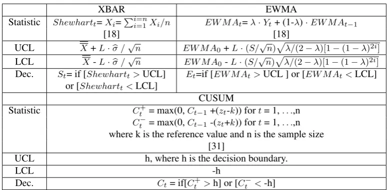
[0,1]describing the weight given to the most recent subgroup mean andLdenoting the rational subgroup standard devia-tion in the control limits (CLs) and it is generally set at3. An illustration of EWMA chart in a simulated dataset is given in Figure (1). Table (2) details formulas about the charting statistics and the CLs as well as the output decision.

3.2 XBAR chart

The Shewhart chart was introduced by [13]. It monitors the process over time based on the mean of the series of in-stances called subgroups. It is a time based chart which sto-res the process history over time. Shewhart-XBAR charts are efficient in detecting large shifts but not small ones. Figure (1) provides an illustration and detailed formulas of XBAR chart. More discussion of these charts will be provided in the next Section.

3.3 CUSUM chart

The CUSUM chart was first introduced by [14]. Then, [15], [16] and [17] developed its mathematical principles. CUSUM is an efficient alternative to Shewhart procedures. It was constructed to overcome shortcomings of Shewhart CCs. It is well suited for small and moderate mean shift detection thanks to its cumulative sum function. Equations and illus-trative plots are given in Table (1) and Figure (1) respectively. We mention thatSt,EtandCtmentioned in Table (1) are the

(3)

[image:3.595.110.501.103.294.2]

Table 1.Properties of three control charts.

XBAR EWMA

Statistic Shewhartt=Xi=Pii==1nXi/n EW M At=λ·Yt+ (1-λ)·EW M At−1

[18] [18]

UCL X+L·_bσ /√n EW M A0+L·(S/√n)pλ/(2−λ)[1−(1−λ)2i_]

LCL X-L·σ /_b √n EW M A0-L·(S/√n)pλ/(2−λ)[1−(1−λ)2i_]

Dec. St= if [Shewhartt>UCL] Et=if [EW M At>UCL ] or [EW M At<LCL]

or [Shewhartt<LCL]

CUSUM

Statistic C_t+= max(0,Ct−1+(zt-k)) fort= 1,. . .,n

C_t−= max(0,Ct−1-(zt+k)) fort= 1,. . .,n

where k is the reference value and n is the sample size [31]

UCL h, where h is the decision boundary.

LCL -h

Dec. Ct= if[Ct+>h] or [C

−

t <-h]

4 Problem of individual charts

appli-cation and motivation

Generally CCs have two important aims. First, they are used as a tool to maintain process stability and control. Thus practitioners have to identify the best CC for any monitoring situation. Second, CCs represent a data analysis tool and le-arning from the process history behavior over time. Despite their performance, individual CCs suffer from some weak-nesses. In this paper, we are interested in improving the formances of CUSUM, EWMA and XBAR charts. The per-formance and the gain obtained by each CC depends on the shift size. To evaluate the CC’s performance, first simulated results are based on a normal distribution with meanµ = 1 and a standard deviationσ=1and we have simulated diffe-rent shift ranges. Figure (2) provides the best selected me-asure of performance of each CC.We base our analysis in terms of different evaluation metrics defined as follows:

True Positive (TP) : It happens when a test signals an

alarm in the process when it is not there (true detection).

True Negative(TN) : It happens when a test signals an

alarm when it is there.

False Positive (FP) : It happens when a test signals an

alarm in the process when it is not there (false detection): type I errors.

False Negative(FN) : It happens when a test does not

signal an alarm when it is there (misdetection): type II errors.

Recall : True Positive Rate.

Accuracy : is computed as follows:

Accuracy=(T P+T N)

N , (1)

where N is the total of the population.

Precision : is the positive predicted rate and it is

com-puted as follows:

P recision= T P

(T P+F P) (2)

F-measure : Is the harmonic mean of precision, and

Re-call and is computed as follows:

F = 2 precisionrecall

(precision+recall) (3)

In fact, each CC’s performance is highlighted in terms of one or more measures but not all. CUSUM’s performance is highlighted in terms of Accuracy and False Positives (FPs). In EWMA, Accuracy and False Negatives (FNs) are the best performance features whereas Recall and FNs are the best performance features for XBAR Chart.

First of all it is obvious that each CC has some advanta-ges and some weaknesses. CUSUM chart has higher accu-racy and smaller FP for small values of shift levels showing a good performance for small shift detection. Nonetheless, it has low performance in detecting moderate and large shifts. This is explained by high FN and small accuracy for mode-rate and large shifts.

The out of control scenario is modelled as follows:µ1=µ0+

δ σ0, whereµ1is the new mean after the shift has occurred,

(4)

[image:4.595.285.525.206.719.2]

to0.96, respectively. Also, the ability to reduce the FPs in CUSUM chart while detecting a small shift is more pronoun-ced. For a shift of1, CUSUM has a FP rate of0.12versus a FP of0.93for a shift of4. This is explained by the fact that the charting statistic of CUSUM chart is based on the cumu-lative sum which makes the detection of small shifts faster. Additional to the weakness of large shift detection, CUSUM has another drawback related to the difficulty to analyze point patterns when all points are highly correlated. Recall and FN measures do not show the effect of CUSUM chart in perfor-ming detection of small shifts, that’s why we only present the most relevant features of performance.

Figure 1. Illustative plots of individual EWMA, CUSUM and Xbar charts monitoring aN(1,1) with a shift in the mean of0.5.

On the other hand, XBAR chart is unable to detect small

shifts. This effect is shown in terms of recall and FNs, where XBAR has a small recall measure when detecting a small shift. However this measure increases for moderate and large shifts. FP also reflects this positive reaction to moderate and large shifts. As an example, when detecting a shift of 1, XBAR registers a recall measure of0.2and an FN of0.8 com-pared to0.99and1when detecting a shift of3.

Figure 2. Individual charts ’s shortcomings in terms of different perfor-mance measures where (a) CUSUM chart, (b) EWMA chart and (c) Xbar chart based onN(1,1) using400observations.

[image:4.595.42.272.255.722.2]

(5)

another disadvantage that each new point in the monitored process depends only on one subgroup of the data without considering the process history. Moreover, EWMA chart is better in detecting small and moderate shifts than large ones. This is shown in Figure 2 in terms of accuracy and FP. A small decrease in the accuracy and an increase in the FP are shown for large shifts. For example, an accuracy of0.815

when a shift is1decreases by more than0.2when detecting a shift of4. Also, the FN rate increases from0.15to0.36for a shift of0.25and3.5, respectively.

While being relatively good in detecting different shift va-lues, CUSUM is still better than EWMA and XBAR in de-tecting small shifts whereas XBAR is better than EWMA and CUSUM in detecting large shifts. The reason of that is that CUSUM chart depends on the entire history of the process making the small shift detection easier. However, Xbar de-pends only on the last subgroup of the data process improving its ability to detect large shifts, while EWMA is a weighted sum of the recent history. Given these conclusions, we need to find a combination of these different CCs. Because each CC has specific advantage and knowledge. Our aim is to be-nefit from all these advantages and competencies in detecting several shift ranges. Also, another aim of our approach is to ease the analysis of monitoring a process through the use of dynamic learning control model.

5 Classification of the time varying

shift for control

Time varying shift detection presents a serious issue in SPC because it requires a dynamic learning monitoring mo-del as well as a re-designing identification system. Although many machine learning methods were integrated into SPC charts, in order to facilitate the shift identification and to as-sign a new competence of shift cause identification, the de-tection of time varying shift in nonstationary environment is still a common issue in SPC. In fact, many techniques use machine learning to improve the identification of special cau-ses of process shift are proposed in the literature.

[19] and [20] have proposed the use of an hybrid ensem-ble learning model to monitor both the mean and variance simultaneously. A combination of the prediction of several artificial neural networks was proposed by [21] to improve the wind speed and power forecast in the context of a weat-her prediction application.

Machine learning algorithms were proposed by [22] through using a neural network and a support vector machine to detect a shift in the mean and to determine variable causes of the control. One of the shortcomings of these methods is that learning models were separately applied. Also, the used learning method is not adapted to the process with time va-rying shifts being based on a fixed learning approach. Many other works have handled SPC shift monitoring problems but without considering the time varying shift and the dynamic nature of the required learning approach to be applied.

Accordingly, all previous methods did not use a dynamic learning model for re-learning and re-designing the time

va-rying shift level. Also, ensemble methods which are designed to cope with shift and concept drift detection were never ap-plied to SPC. That’s why, our aim is to propose a method that has at least three advantages: (1) to use dynamic classifica-tion methods that can learn the shift and adapt the model to the time varying magnitude of the process change, (2) to ag-gregate decision from several CCs used simultaneously using an ensemble method for non stationary environment (3) to propose a method that is able to detect both small and large shifts.

In fact, this research is based on a general set up that works with little number of required information. The most impor-tant and only information needed is online data with zeros and ones as class labels, where0indicates that the batch or the instance has been correctly classified whereas 1 indica-tes that the batch or the instance has been wrongly classified. The properties we have to comply with are described in the following points: (a) the data can be in forms of instances or batches, (b) the required information is the classification error rates, (c) the change to be detected can be sudden or gradual, (d) specific or ensemble method can be used and (e) attributes charts or variable charts can be used.

6 Dynamic ensemble CC model

6.1 Data set assessment of the ensemble

met-hod

In order to minimize the risk of choosing a non adequate CC, as well as to enhance the detection of concept drift, an ensemble of CCs is used instead of choosing the best one. The idea of using adaptive techniques to detect concept drift is inspired from machine learning techniques such as STAG-GER of [23], DWM of [24] and [25], DWM-WIN of [7], SVM of [26] and IFCS of [27]. An adaptive combined chart is developed based on a weighted majority vote over the dif-ferent classifers’ decisions of the CCs for each instance of the batch. We use the DWM of [24] and DWM-WIN of [7] to get this class prediction about the learned shift. Algorithm (1) defines these steps.

In Step1, the dataset of the DEC chart model is based on the combination of the charting statistics ofkindividual CCs. The proposed method is suitable to be applied to all CCs ty-pes. Each charting statistic is presented in a vectorXk. Then,

the different vectors are concatenated and stored in a matrix calledXkfork=1,. . .,pgiven by

Xk=



    

x1k

x2k

.. .

xpk



    

(4)

wherepis the number of CCs,Xkis the charting statistics

(6)

Algorithm 1:Combined chart model based on Dyn-amic weighted majority algorithm for drift detection.

1: Inputsp: Initialize number of CCs to monitor the

process.

β: parameter for decreasing classifier’s weight when state decision is correct.

η: parameter for increasing classifier’s weight when state decision is incorrect.

θ: threshold for removing classifiers from the ensemble

2: Step1:Data Pre-processing

1.1: Apply p chart for each batch of data

1.2: Store the charting statistics of each chart in vectors

X1,X2,. . .,Xp.

1.3: Concatenate vectorsXnin a matrix of p columns:

this represents the combined data D.

3: Step2:Apply DWM-WIN algorithm to combine chart’s decisions.

2.1 Initialize classifier’s weights.

2.2 Apply DWM to the new generated data D

2.3 Compute the error rates of DWM-WIN based on D

XShewhart=

      x11 x21 .. .

xk1

     

, XCusum=

      x12 x22 .. .

xk2

     

, Xewma=

      x13 x23 .. .

xk3

      (5) Equations (4)-(9) describe the different sub-steps of the pre-processing data phase.

For a combination of3CCs, the new data will be

X3=      

x11 x12 x13

x21 x22 x23

..

. ... ...

xk1 xk2 xk3

      (6)

More generally, the dataset representing the combination ofpcharts is:

Xp=          

x11 x12 x13 . . . x1p

x21 x22 x23 . . . x2p

xm1 xm2 xm3 . . . xmp

xm1+1 xm2+1 xm3+1 . . . xmp+1

..

. ... ... . .. ...

xk1 xk2 xk3 . . . xkp

          (7)

The next pre-processing step consists on applying DWM algorithm to the generated data in order to monitor its clas-sification error rates and to detect the shift in the data. This is done through a simultaneous use of more specific know-ledge about the data by using the charting statistics informa-tion and the DWM as a technique of concept drift detecinforma-tion. We simultaneously base our experiments on data with diffe-rent shifts in the mean aiming to prove the detection ability of the combined CC versus single charts in detecting concept drift during the classification process. To apply DWM, class

labels have to be defined. Thus, before the shift occurs in the process we assume that the class label is 0. Then, when a shift occurs, the class label is 1. Forpvariables, if the shift occurs in observation k

2+1the class label will be as follows:

Classlabel=             0 0 0 .. . 1 1 1             (8)

Finally, the new data is:

X=            

x11 x12 x13 . . . x1p 0

x21 x22 x23 . . . x2p 0

xm1 xm2 xm3 . . . xmp 0

xm1+1 xm2+1 xm3+1 . . . xmp+1 1 xm1+2 xm2+2 xm3+2 . . . xmp+2 1

..

. ... ... . .. ... ...

xk1 xk2 xk3 . . . xkp 1

            (9)

DWM is called to detect the concept drift. More precisely, each classifier will initially have a weight of one. The weight of classifiers will be decreased if the classifier predicts in-correctly the state of the process based on the ensemble of chart’s statistics and increased if the classifier’s global pre-diction is correct. This step will be applied for the three CCs until having three final weights. If the weight of each CC is under the thresholdθ, the classifier will be removed from the ensemble, else it will be maintained. Then, a global pre-diction vector will be computed from the remaining ensemble of classifiers. When this global prediction of classifiers based on the CC decisions is wrong, a new classifier is added. The same reasoning would continue until finding the best combi-nation of classifiers which detects if the process is in control or out of control for the different batches of the process. The size of the batch affects the detection of the shift via the mis-classification error rates. A shift could either be detected or absorbed by the system. In fact, for large batch sizes, the shift is detected and considered while updating the weights inside one batch. However, for small batch sizes, the shift induces a high error which is expected to be more obvious with the monitoring method.

7 Experiments

7.1 Simultaneous small and large shift

de-tection

(7)

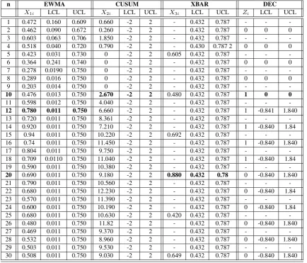
on two datasets, with a small shift in the mean of0.25and a large shift of3.5, are simulated to illustrate the proposed mo-del. The dataset consists of30observations where the shift in the mean occurs in observation11. Therefore, the first 10 observations are simulated based onN(0.5,0.52) in both da-tasets and the second20observations are simulated based on aN(0.75,0.52) andN(4,0.52) in the first and the second ex-ample respectively. First data is denotedD1and is shown in Table (2) and second data is denotedD2and is shown in Ta-ble (3). The charting statistics of EWMA, CUSUM, XBAR and DEC charts areX1i,X2i,X3i andZi respectively. The

upper and lower CLs of EWMA, CUSUM, XBAR and DEC charts are (LCL1,U CL1), (LCL2,U CL2), (LCL3,U CL3) and (LCLz, U CLz) respectively. Tables (2) and (3)

sum-marize the results for the different methods using the same random generation numbers denoted ”seed”.

For the first dataset, EWMA and CUSUM chart can detect the shift that occurred in observation11at timet12andt10. However, XBAR detects the small shift inD1in observation

20. One reason of XBAR’s delay to detect the small shift is that its charting statistic is based on an independent subgroup of the dataset which decreases the ability of a quick small shift identification. For DEC chart, the shift is detected by the increase in the misclassification error rates. Then, the DWM algorithm needs some time to update the internal knowledge after the shift detection by removing and adding of experts as well as weight adjusting and other steps. All these steps re-quire some time before reaching a certain stability which can be shown when the error goes back to0. This explains how the shifts are detected and how the errors are failing back to0

after a while. Furthermore, thanks to its prediction ability our proposed method has an immediate detection ability explai-ned by the use of classification methods which eases the shift prediction from observation10. Accordingly, DEC chart is as good as CUSUM chart but much faster than EWMA and XBAR in detecting small shift range.

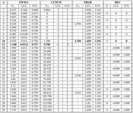
For the second dataset with large shift in the mean, a shift in the last20observations is also simulated. According to Ta-ble (3), DEC model is as good as Xbar chart to identify such shift. It predicts, identifies the shift at observation10thanks to the learning classification methods aggregating the decisi-ons of the ensemble of charts’ decision, EWMA detects it at

t11, CUSUM att11and XBAR att10. As expected, XBAR has an early detection ability compared to EWMA and CU-SUM to detect such shift inD2.

This advantage is explained by the use of the misclassifica-tion error rates as charting statistics of the monitoring process in DEC chart.

7.2 Improvement of the misclassification error

rates

In this section we first concentrate on evaluating the control charts in terms of error of classification which is measured with the misclassification error rates (or type II errors). In the next section, we will compare the CCs ba-sed on other measures of performance such as FPs (error type I), accuracy and recall measures. The reason of that

Figure 3.Shift comparison based on ewma misclassification error rates.

is that the misclassification error rates are very informa-tive about the shift during processes and thus we studies the type II error rates first.

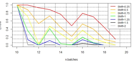
We focus on a shift simulation analysis based on several values of shift parameters. In Figure (3), the error rates of EWMA chart for shift values parameters are plotted based on aN(µ=0,σ=1) of400observations with a shift in the middle. It shows that the change in the error rates of EWMA chart is clearly impacted by the change of the shift level, ex-cept the change point of the shift detection which is practi-cally the same. The relation between the speed of the adapta-tion of the error process after the shift detecadapta-tion and the shift level is clear. Changes in batches13,15and16are random change points which are detected with different levels of er-rors impacted by the level of the shift.

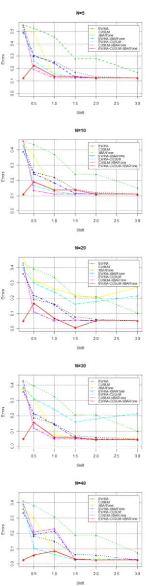
Because the reaction of the chart to the shift is highly infor-mative about the robustness of the method to detect the chan-ges and to adapt itself after the shift detection, we conduct a comparative study between the different variants of DEC chart and the individual charts. Thus, we compare results obtained by the different variants of DEC chart denoted: (1) EWMA-CUSUM, (2) EWMA-Xbar, (3) CUSUM-Xbar and (4) XBAR-CUSUM-EWMA with the application of indivi-dual CCs: EWMA, CUSUM and Xbar. The combined CCs were implemented based on 400observations with a mean shift in the middle using a number of batches of5,10,20,30

and40. The procedure used by DWM algorithm, to divide the data in different batches, train on then−1recent bat-ches and test on the last batch, is the same procedure used for generating a k fold cross validation. The latter consists on portioning the data intonsubsets, performing the training on one subset and test on the other subsets. So, the number of batches is equal to the numberkused to generatekfold cross validations. Indeed, we compute the mean over 10runs for each method. By using this procedure, we abstain sampling biases. Furthermore, we use other measures of performance such as F-measure, recall, FPs ad FNs and statistically com-pare the difference between the methods.

DEC chart is configured with the following parameters: β

[image:7.595.315.542.107.215.2]

(8)

[image:8.595.75.510.125.496.2]

Table 2.Illustrative examples of EWMA, CUSUM, XBAR and ensemble chart model for small shift in the meanδ=0.25inN(0.5,0.52). The first10 observations follow aN(0.5,0.52_{) and the last}₂₀_{observations follow a}_N_{(shift + 0.5,}₀_.₅2_{) using the same set.seed (random number generation). For}

EWMA,λ=0.2andL=3are used and for CUSUM,k=1andh=3.

n EWMA CUSUM XBAR DEC

X1i LCL UCL X2i LCL UCL X3i LCL UCL Zi LCL UCL

1 0.472 0.160 0.609 0.660 -2 2 - 0.432 0.787 - -

-2 0.462 0.090 0.672 0.260 -2 2 - 0.432 0.787 0 0 0

3 0.603 0.063 0.706 1.850 -2 2 - 0.432 0.787 - -

-4 0.518 0.040 0.720 0.790 -2 2 - 0.430 0.787 2 0 0 0

5 0.423 0.031 0.730 0 -2 2 0.605 0.432 0.787 - -

-6 0.364 0.241 0.740 0 -2 2 - 0.432 0.787 0 0 0

7 0.278 0.0190 0.750 0 -2 2 - 0.432 0.787 - -

-8 0.289 0.016 0.750 0 -2 2 - 0.432 0.787 0 0 0

9 0.203 0.014 0.750 0 -2 2 - 0.432 0.787 - -

-10 0.476 0.013 0.750 2.670 -2 2 0.480 0.432 0.787 1 0 0

11 0.598 0.012 0.750 4.040 -2 2 - 0.432 0.787 - -

-12 0.780 0.011 0.750 6.660 -2 2 - 0.432 0.787 1 -0.841 1.840

13 0.720 0.011 0.750 8.361 -2 2 - 0.432 0.787 - -

-14 0.920 0.011 0.750 7.210 -2 2 - 0.432 0.787 1 -0.840 1.84

15 0.94 0.011 0.750 10.220 -2 2 0.692 0.432 0.787 - -

-16 0.74 0.011 0.750 11.450 -2 2 - 0.432 0.787 1 -0.840 1.840

17 0.804 0.011 0.750 9.750 -2 2 - 0.432 0.787 - -

-18 0.709 0.0110 0.750 11.040 -2 2 - 0.432 0.787 1 -0.840 1.84

19 0.590 0.011 0.750 10.380 -2 2 - 0.432 0.787 - -

-20 0.690 0.011 0.750 9.180 -2 2 0.880 0.432 0.78 0 -0.840 1.840

21 0.790 0.011 0.750 10.560 -2 2 - 0.432 0.787 - -

-22 0.680 0.011 0.750 12.230 -2 2 - 0.432 0.787 0 -0.840 1.84

23 0.570 0.011 0.750 11.390 -2 2 - 0.432 0.787 - -

-24 0.600 0.011 0.750 10.190 -2 2 - 0.432 0.787 0 -0.840 1.84

25 0.680 0.011 0.750 10.630 -2 2 0.420 0.432 0.787 - -

-26 0.480 0.011 0.750 11.82 -2 2 - 0.432 0.787 0 -0.840 1.840

27 0.469 0.011 0.750 9.370 -2 2 - 0.432 0.787 - -

-28 0.532 0.011 0.750 8.960 -2 2 - 0.432 0.787 0 -0.840 1.840

29 0.503 0.011 0.750 9.530 -2 2 - 0.432 0.787 - -

-30 0.508 0.011 0.750 9.030 -2 2 0.649 0.432 0.787 0 -0.840 1.840

results by the mean of these iterations. The task of DEC chart is to mine the charting statistics of the different CCs. To treat this problem, DEC proposes a classification task so-lution. It combines many decisions at each time step based on DWM-WIN algorithm to increase the probability of correctly classifying a change point.

Here, we track the degree of diversity of the CC ensem-ble. Thus, we analyze the capacity of the combined CC mo-del based on a normal distribution withµ=0andσ =1by comparing it with the individual chart model in terms of mis-classification error rate of DWM-WIN. For the EWMA chart, many values of the parameterλare used in the literature. In general, values of this parameter are between0and1as sta-ted by [26]. In this experiment,λ=0.2andL=3are used with the notation that these parameters can be optimized. For CUSUM chart we use the decision boundaryh= 4, the refe-rence valuek=1and the target value representing the actual process mean. T =1. For XBAR chart used in this simu-lation, we use the Xbar’one (xbar) chart function from the quality control chart (qcc) R package which computes sta-tistics required by the xbar chart for one at-time data. The reason of this choice is that we need to combine vectors of

charting statistics of equal size. This can only be obtained by the Xbar’one chart where the number of subgroups is equal to the dataset size as in CUSUM and EWMA charts.

In Figure (4), the horizontal axis represents the shift level and the vertical axis the error rates of the classification en-semble method used to combine the different chart models. We base our analysis on 6 shift levels. The analysis is as follows:

Shift =0.25: The differences between methods are more

pronounced for small shift values. Although all other indi-vidual chart models as well as the combined ones: EWMA-CUSUM, EWMA-XBAR and XBAR-EWMA charts begin with relatively high errors, EWMA-CUSUM-XBAR starts with low error rates by perfectly coping with the shift level

0.25. In fact, the ensemble chart model begins with misclas-sification error rates between0.055and0.12for all different number of batches situations, however it is greater than0.4

for individual charts. Thus, our proposed CC outperforms ot-her CCs and is able to track small shifts when considering the statistics information of more than one chart.

Shift =0.5: When the shift level is0.5, errors of the

(9)

[image:9.595.91.520.123.488.2]

Table 3.Illustrative exmaples of EWMA, CUSUM, XBAR and ensemble chart model for large shift in the mean of3.5inN(1,1). The first10observations follow aN(0.5,0.52_{) and the last}₂₀_{observations follow a}_N₍₀_.₅_{+ shift,}₀_.₅2_{) using the same set.seed (random number generation). For EWMA,}_λ₌₀_.₂

andL=3are used and for CUSUM,k=1andh=3.

n EWMA CUSUM XBAR DEC

X1i LCL UCL X2i LCL UCL X3i LCL UCL Zi LCL UCL

1 0.472 0.160 0.609 0.084 -2 2 - 2.450 3.101 - -

-2 0.460 0.090 0.672 0 -2 2 - 2.450 3.101 0 0 0

3 0.603 0.063 0.706 0 -2 2 - 2.450 3.101 - -

-4 0.518 0.043 0.726 0 -2 2 - 2.450 3.101 0 0 0

5 0.420 0.031 0.738 0 -2 2 2.550 2.450 3.101 - -

-6 0.360 0.024 0.740 0 -2 2 - 2.450 3.101 0 0 0

7 0.270 0.019 0.746 0 -2 2 - 2.450 3.101 - -

-8 0.289 0.0160 0.751 0 -2 2 - 2.450 3.101 0 0 0

9 0.203 0.016 0.754 0 -2 2 - 2.450 3.101 - -

-10 0.470 0.014 0.756 1.580 -2 2 2.350 2.450 3.101 1 0 0

11 1.240 0.0132 0.757 8.700 -2 2 - 2.450 3.101 - -

-12 1.950 0.012 0.750 16.740 -2 2 - 2.450 3.101 1 -0.090 1.690

13 2.450 0.011 0.758 24.090 -2 2 - 2.450 3.101 - -

-14 2.640 0.011 0.758 29.320 -2 2 - 2.450 3.101 1 -0.090 1.690

15 3.106 0.011 0.759 37.650 -2 2 2.642 2.450 3.101 - -

-16 3.340 0.011 0.759 44.660 -2 2 - 2.450 3.101 1 -0.090 1.690

17 3.310 0.011 0.759 49.470 -2 2 - 2.450 3.101 - -

-18 3.509 0.011 0.759 56.520 -2 2 - 2.450 3.101 1 -0.090 1.690

19 3.52 0.011 0.759 62.122 -2 2 - 2.450 3.101 - -

-20 3.49 0.011 0.759 67.305 -2 2 2.830 2.450 3.101 1 -0.090 1.690

21 3.66 0.011 0.759 74.420 -2 2 - 2.450 3.101 - -

-22 3.810 0.011 0.759 81.750 -2 2 - 2.450 3.101 1 -0.090 1.690

23 3.75 0.011 0.759 87.210 -2 2 - 2.450 3.101 - -

-24 3.680 0.011 0.759 92.390 -2 2 - 2.450 3.101 0 -0.090 1.690

25 3.740 0.011 0.759 98.810 -2 2 3.022 2.450 3.101 - -

-26 3.840 0.011 0.759 105.790 -2 2 - 2.450 3.101 0 -0.090 1.690

27 3.650 0.011 0.759 110.040 -2 2 - 2.450 3.101 - -

-28 3.660 0.011 0.759 115.820 -2 2 - 2.45 3.101 0 -0.090 1.690

29 3.730 0.011 0.759 122.330 -2 2 - 2.450 3.101 - -

-30 3.710 0.011 0.759 128.304 -2 2 - 2.450 3.101 0 -0.090 1.690

On the other hand, all combined two chart models: EWMA-CUSUM, EWMA-XBAR and CUSUM-XBAR perform bet-ter than individual charts for all batch size situations. For example, forN=5, these methods greatly outperform indivi-dual charts. This is due first to the advantages of the ensemble method technique over the individual ones. Second, this per-formance is also due to the fact that statistics used for each CC are very informative about the quality control of process behavior. Also, the DWM-WIN used in the combined chart models allows this technique to easily detect shifts in the pro-cess and to update the internal knowledge announced in the CC about this shift.

Shift =1: For this shift level, errors of individual charts

decrease compared to smaller shift level situations because all these CCs are more sensitive to detect large shifts, except the CUSUM which is based on accumulating changes in one direction and hence is more sensitive to small shifts. Com-bined models are still more robust to react to the shift better than individual charts. XBAR, CUSUM and EWMA do not show this effect in detecting shifts in processes because the internal information does not allow it. More rigorously, the combined chart model performs better than other individual charts, in particular XBAR-CUSUM and EWMA-CUSUM

are the best ones for N = 10and N = 30. This is due to the fact that CUSUM chart is more sensitive to small shifts and EWMA and XBAR perform better with large shift cases as explained earlier. Thus, combining CUSUM with XBAR and with EWMA outperforms the decision of only one chart model in detecting a shift of1.

Shift =1.5: All CC error rates decrease when the shift level

increases to1.5. In particular, EWMA-CUSUM-XBAR chart errors are between0.05and0.12whereas other charts reach error rates of0.2and even more forN=5. An error rate of

0.28is obtained with XBAR chart. More precisely, XBAR-CUSUM shows a good reaction capacity to shift detection for all batch size situations. This is due to the combined effect of the two charts and the diversity of the internal knowledge gi-ven by the two different charts, one is sensitive to very small shifts and the other is more sensitive to large shifts.

Shift = 2 Combined EWMA-CUSUM-XBAR chart

out-performs other CCs for moderate and large shifts. In fact, it has a maximum error of 0.12, individual charts reach0.28, two combined models reach0.18forN=30.

Shift =3: Similar results are obtained as for shift level =

2.

(10)

EWMA-Figure 4. Comparison of the misclassification error rates of DWM-WIN monitoring the different combined control chart models versus the individual charts for a variety of shift levels.

CUSUM-XBAR chart outperforms individual CCs. When the diversity of combined CCs increases, the

misclassifica-tion error rates decrease accordingly. When combining three CCs based on a dynamic ensemble method for concept drift, the accuracy of the CC improves. As shown in Figure 4, EWMA-CUSUM-XBAR chart depicts smaller values of mis-classification error rates better than the combined two chart model. Interestingly, the diversity in combining CCs pre-sents an important factor to improve the classification accu-racy rate of the proposed chart in both monitoring small and large shifts in the mean.

8 Comparison of DEC chart with

combined SFEWMA-X chart

[image:10.595.85.236.84.688.2]

In this section we focus on comparing the proposed dyn-amic chart DEC with one of the combined charts from the literature called Single Featured EWMA chart (SFEWMA-X) of [29].

Figure 5. Performance evalutioon of proposed DEC chart model versus combined SFEWMA-X chart based onN(µ=1,σ2₌₁_{) using 400}

obser-vations.

Like DEC chart, the latter was proposed with the aim to both monitor small and large shifts in the process.SFEWMA chart was proposed to handle the problem of combining EWMA-X chart of using two sets of statistics and CLs by proposing only one set of statistic and CLs. This method aims to identify both small and large shifts. The basic idea of SFEWMA-X is to transform the EWMA statistic into a new one in order to have the same scale for Shewhart-X and EWMA charts. This is done by performing a variable transformation called ”multiplyer” to rescale the statistic of EWMA into the same range of the statistic of Shewart-X chart and thus make the application of the combined chart easier. The main raison of choosing this method among others is because it is similar to our method in the

idea of unifying the statistics of CCs. In their article, [29]

compared SFEWMA-X only to individual charts. Here, we compare SFEWMA-X to individual charts and also the pro-posed DEC chart. Comparisons were conducted in terms of errors and in terms of different performance measures. Fi-gure (5) compares error rates of DEC chart and SFEWMA-X chart for the different shift sizes.

[image:10.595.311.527.317.458.2]

(11)

increa-ses, DEC’s error decreases until achieving a stable level of error of0.11for shifts ranging from0.75to4. Concerning SFEWA-XBAR chart, the error is decreasing until a shift of

1.5achieving0.13of error. Then, it increases again to achieve

0.25for shift2.5until4. Thus, the performance of dynami-cally combining three CCs based on DWM algorithm outper-forms the SFEWMA-X chart. The reason for that is that first, DEC chart uses more statistical information than SFEWMA-X chart. Second, the dynamic combination through the use of DWM algorithm is much more informative about the shift detection points than the use of the rescaled parameter propo-sed to combine EWMA and XBAR in SFEWMA-X. Indeed we note that the decrease in the error is impacted by the shift level. This is explained by the relation between the know-ledge about the shift level and the classification errors. In fact, a clear knowledge about the shift, obtained by higher levels, impacts the classification errors. Thus, the clear is the knowledge representation of the shift obtained, the smaller is the classification error. This reasoning is confirmed by [30] when they show the high relation between the knowledge-based levels and the error of classification.

[image:11.595.318.553.86.264.2]

To go further in our analysis, we want to understand the cause of high errors in SFEWMA-X compared to DEC chart. Thus, we concentrated on the behavior of the two charts for shifts smaller than1. Figure (6) shows the high differences in errors between the two methods based on the mean over the Type I and Type II errors.

Figure 6. Boxplot comparing the mean over Type I and Type II errors of DEC chart and SFEWMA-X charts based on100runs.

As noticed, the variance in SFEWMA-X is higher than in DEC chart for shift of1. Compared to SFEWMA-X chart, the DEC chart is more stable in results and procures smaller error variance.

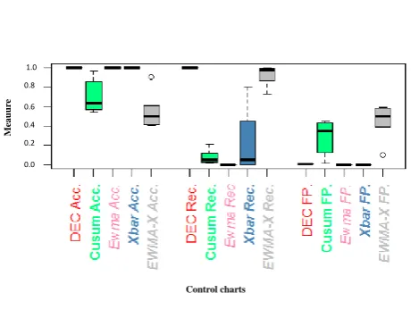
To go further in our analysis, we compare DEC chart with SFEWMA-X as well as individual CUSUM, XBAR and EMWA charts in terms of accuracy, recall and FP measures. Figures (7) to (9) show the comparisons of performances of the different methods for small-moderate and large shifts.

The performance of each method could be highlighted ba-sed on one measure and not the others. Each measure is sen-sitive to evaluate one or more methods but not all of them.

0.0 0.2 0.4 0.6 0.8 1.0

M

ea

uur

e

Control charts

Figure 7. Performance evaluation of DEC model compared to individual EWMA, CUSUM and Xbar in terms of Accuracy, Recall, FP and FN rates: small-moderate shifts.

That’s why, instead of error rates, we use accuracy, FPs and FNs. For small and moderate shifts as shown in Figure (7), DEC chart outperforms SFEWMA-X and individual charts in terms of accuracy, recall and FP rates. SFEWMA-X is com-petitive with respect to DEC chart and outperforms individual EWMA and XBAR in terms of recall. The performance of CUSUM chart is not highlighted here because of the low per-formance of this type of chart in detecting the moderate shift which is included in the computations done in the boxplots.

0.0 0.2 0.4 0.6 0.8 1.0

M

ea

uur

e

[image:11.595.59.298.444.601.2]

Control charts

Figure 8. Performance evaluation of DEC model compared to individual EWMA, CUSUM and XBAR in terms of Accuracy, Recall, FP and FN rates: large shifts.

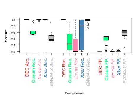
[image:11.595.317.552.450.618.2]

(12)

the moderate shift included in the computations done in Fi-gure (8). DEC chart’s performance is noticed through the different measures and a high robustness and stability to the shift detection than the combined SFEWMA-X chart as well as when compared to other individual charts.

0.0 0.2 0.4 0.6 0.8 1.0

M

ea

uur

e

[image:12.595.44.269.163.338.2]

Control charts

Figure 9. Performance evaluation of DEC model compared to individual EWMA, CUSUM and Xbar in terms of Accuracy, Recall, FP and FN rates: all shifts.

Figure (9) illustrates a summary for more general results over the different shift sizes. SFEWMA-X outperforms in-dividual EWMA and XBAR and is as good as DEC chart in terms of Recall. However, this effect is not shown in terms of accuracy and FP rates. Being already very performant to shift detection, this method assumes that the class labels are unknown. In the next chapter, we propose a new combined chart without the assumption of known classes in order to make the application in real word data possible.

9 Conclusions

The proposed CC does not only exhibit superior robustness to individual EWMA, CUSUM and XBAR for some perfor-mance measures but also presents a new heuristic for shift learning and monitoring in nonstationary environment. DEC chart presents the second CC proposed by aggregating the de-cisions of three different CCs based on DWM method after DWMCC. Results show that the use of the ensemble techni-ques in CCs outperforms the use of single CCs as well as other combined charts when several shift levels have to be monitored in terms of different measures thanks to the fact that the use of DWM in CCs allows an identification of the shift learning process. In order to enable the application of combined charts to real world data, a new model based on both DWM-WIN as well as TACL chart was proposed. In fact, DWM was used in learning while monitoring with CCs by applying exactly the same mechanism dealing with classi-fiers in the DWM to CCs. Using this new heuristic of treating CCs as classifiers by adding, removing and dynamic weig-hting of CCs based on their performance leads to a better

shift identification ability. Results show that the DWM chart model leads to the best model to deal with the non stationa-rity of the data compared to models from the most successful individual SPC techniques. This article presents the appli-cation of the method on different simulated scenarios of non-stationarity processes and on time varying processes. An interesting extention of this article would be to apply this method to a real dataset and to study the relationship between the process variability and the type of charts to be combined.

Another possible perspective to this research is that instead of applying many CCs to one dataset and combining the deci-sion over the different charts, one can apply one CC to diffe-rent features of the data, then combine the decision over the different features. This would represent a new multivariate application of ensemble methods in SPC.

REFERENCES

[1] D. Mejri, M. Limam, and C. Weihs, (2016), ” A new dynamic weighted Majority Control chart for data streams”, Journal of Soft Computing, DOI: 10.1007/s00500-016-2351-3, pp:1-12.

[2] M. R. R., Jr and G.-Y., Chob, (2011). Multivariate control charts for monitoring the mean vector and covariance matrix with variable sampling intervals. Sequential Analysis: Design Methods and Applications, 30(1):140.

[3] M. R. S. Z. G., Reynolds, JR., (2008). Combinations of mul-tivariate shewhart and mewma control charts for monitoring the mean vector and covariance matrix. Qulaity Technology, 40(4):381393.

[4] D. Zeng, I. Gotham, K. Komatsu, C. Lynch, M. Thurmond, D. Madigan, B. Lober, J. Kvach, and H. Chen, (2007). Intel-ligence and Security Informatics : Biosurveillance. Second NSF Workshop, New Brunswick, NJ, USA, Proceedings, vol. 4506 of Lecture Notes in Computer Science. Springer.

[5] J. C. Brillman, T. Burr, D. Forslund, E. Joyce, R. Picard, and E. Umland, (2005). Modeling emergency department visit patterns for infectious disease complaints: results and application to disease surveillance. BMC medical informatics and decision making, 5:4.

[6] B. Y. Reis, and K. D. Mandl, (2003). Time series modeling for syndromic surveillance. BMC medical informatics and decision making, 3:111.

(13)

[8] H. Wang, W. Fan, P. S. Yu, and J. Han, (2003). Mining concept-drifting data streams using ensemble classifiers. In Proceedings of the Ninth ACM SIGKDD International Conference on Knowledge Discovery and Data Mining, KDD 03, pages 226235, New York, NY, USA. ACM.

[9] H. B. Nembhard, and M. S. Kao, (2003). Adaptive forecast based monitoring for dynamic systems. Technometrics, 45(3):208219.

[10] X. Zhang, I. Elishakoff, and R. Zhang, (1991). A Stochastic Linearization Technique Based on Minimum Mean Square Deviation of Potential Energies. Springer Verlag.

[11] M.C. Georgiadis, J. R. Banga, and E. N. Pistikopoulos,

(2010). Dynamic process modeling: Combining models

and experimental data to solve industrial problems. Process Systems Engineering: Dynamic Process Modeling, 7:208219.

[12] S. W. Robert, (1959). Control chart test based on geometric moving average. Technometrics, 42(1):97102.

[13] W. A. Shewhart, (1931). Economic Control of Quality

of Manufactured Product. New York: D. Van Nostrand

Company.

[14] E. S. Page, (1954). Continuous inspection scheme. Biome-trika, 41(1/2):100115.

[15] W. D. Ewan, (1963). When and how to use cusum charts. Technometrics, 5(1):122.

[16] N. L. Johnson, (1961). A simple theoretical approach to cumulative sum control chart. Journal of the American Statistical Association, 56(296):835840.

[17] N. L. Johnson, and F. C. Leone, (1962). Cumulative sum control charts: Mathematical principles applied to their construction and use, part i. Industrial Quality Control, 18(12):1521.

[18] D. Montgomery, (2005). Introduction to Statistical Quality Control. 5th edition, New York: John Wiley and Sons.

[19] W. Yang, Y. G. and W. Liao, (2015). A hybrid learning based model for simultaneous monitoring of process mean and variance. Quality Reliability Engineering, 31:445463

[20] B. Wu, and J.B. Yu, (2010). A neural network ensemble mo-del for online monitoring of process mean and variance shifts in correlated processes. Expert Systems with Applications, 37(6):4058–4065.

[21] Z. Men, E. Yee, F.S. Lien, Z. Yang, and Y. Liu, (2014). Ensemble nonlinear autoregressive exogenous artificial

neural networks for short term wind speed and power fore-casting. International Scholarly Research Notices, ID 972580.

[22] C. S. Cheng, and H. P. Cheng, (2008). Identifying the source of variance shifts in the multivariate process using neural networks and support vector machines. Expert Systems with Applications, 35(1-2):198206.

[23] J. C. Schlimmer, and R. H. Granger, (1986). Beyond incre-mental processing: Tracking concept drift. In Proceedings of the Fifth National Conference on Artificial Intelligence, pages 502507. AAAI Press, Menlo Park, CA.

[24] J. Z. Kolter, and M. A. Maloof, (2007). Dynamic weighted majority: An ensemble method for drifting concepts. Journal of Machine Learning Research, 8:2755 2790.

[25] J. Z. Kolter, and M. A. Maloof, M. A. (2005a). Dynamic weighted majority: A new ensemble method for tracking concept drift. In International Conference on Data Mining (ICDM), pages 123130. IEEE.

[26] S. N. Ahmed, L. Huan, and S. K. Kay, (1999). Handling concept drifts in incremental learning with support vector machines. In Proceedings of the Fifth ACM SIGKDD International Conference on Knowledge Discovery and Data Mining, KDD 99, pages 317 321, New York, NY, USA. ACM.

[27] J. Schlimmer, and R. Granger, (2011). Fuzzy classification in dynamic environments. Soft Computation, 15(5):10091022.

[28] S. H. Steiner, (1999). Ewma control charts with time-varying control limits and fast initial response. Journal of Quality Technology , 31(1):7586.

[29] C. S. Liu, and F. C. Tien, (2010). Design of single featured ewma x control chart for process mean shift detection. In Proceedings of the 2nd International conference on Applied Operational research, pages 301314. Lecture Notes in Management Science.

[30] H. Pasman, (2015). Risk Analysis and Control for Industrial Processes - Gas, Oil and Chemicals. A System Perspective for Assessing and Avoiding Low-Probability, HighConsequence Events. Elsevier Science.