"Lazy" Wavelets of Hermite Quintic Splines and a
Splitting Algorithm
Boris M. Shumilov
1,*, Ulukbek S. Ymanov
21Applied Mathematics Department, Tomsk State University of Architecture and Building, Tomsk, 634003, Russia 2Business & Management Faculty, Osh State University, Osh, 723500, Kyrgyzstan
*Corresponding Author: [email protected]
Copyright © 2013 Horizon Research Publishing All rights reserved.
Abstract In this article two new types of wavelet bases
for Hermite quintic splines are offered. The algorithm of wavelet decomposition as the solution of three systems of the linear equations, from which one system is three-diagonal with strict diagonal domination and two other systems are four-diagonal, is received.Keywords Hermite Splines; Wavelets; Relations of
Decomposition and Restoration1. Introduction
Wavelet refers to as small, i.e. the short (with compact support) or quickly fading wave, which hierarchically organized compressions and displacements form a set spanning some space of the bounded functions on the whole numerical axis [1-3]. At the expense of compression wavelets reveal with a different degree of a detail distinction in the characteristics of the measured signal, and by displacement are capable to analyze properties of a signal in different points on the entire investigated interval. As against Fourier transformation, which gives only global information on properties of a researched signal, as the basic functions used at it (sine and cosine) are supported on the unbounded interval, the wavelets provides essential advantage at the analysis of non-stationary signals. At the solution of tasks of the numerical analysis, as wavelets will transform system of basic functions with the distributed parameters to system with the concentrated parameters, such basis appears much more effective from the point of view of conditionality and convergence. As to orthonormal and bi-orthogonal wavelets [1] they have not analytical representation and graphically are similar to fractal curves. Semi-orthogonal spline wavelets [2] are deprived these defects, that makes them convenient for use in interpolating graphical objects [3]. However defect is that these wavelets are supported on the rather wide interval.
In a number of works [4-9] the reduction of supports was achieved by construction of Hermite spline multi-wavelets,
at which more than one basic function are associated to each node. In given article, using this idea, we shall construct basic wavelets on space of Hermite splines of the fifth degree. Along with classical one, we shall consider unknown type of «lazy» multi-wavelets and we shall prove the new approach to calculation of wavelet transformation on the base of the finite implicit relations of decomposition with splitting at even and odd nodes.
2. Examples of Systems of «Lazy»
Hermite Quintic Spline Wavelets
2.1. Hermite Quintic Splines
The starting point for construction of wavelet transformation is the nested set of vector spaces … VL–1⊂ VL
⊂ VL+1 …. In our case VL is a space of splines of a degree 5
smoothness C2 on an interval [a, b] with an uniform grid of nodes ΔL : u
i = a + (b – a) i / 2L, i = 0, 1,…, 2L, L ≥ 0, and
basic functions NL
i,k (v) = φk (v – i), k = 0, 1, 2 ∀i, where
v = 2L (u – a)/ (b – a)+ 1, with the centers in integers are
scaling’s and translations of three functions of a kind (Figure 1):
3 2 3 2 3
2 0
1
3 2 2
3 2 3
2
(6 15 10)
(3 7 4) ,0 1;
( ) ( 2 1)
2
( ) ,
( ) (2 ) (6 9 4)
(2 ) (3 5 2) ,1 2;
(2 ) ( 2 1) 2
( ) 0,
k
t t t
t t t t
t
φ t t t
φ t
φ t t t t
t t t t
t t t
φ t k
− +
− − + ≤ ≤
− +
=
− − +
− − + ≤ ≤
−
− +
= =0,1, 2,t∉[0,2].
On any grid ΔL, L ≥ 0, interpolating Hermite spline of the
5-th degree can be expressed as
( )
2 2 ,( )
, 0 0
, ,
L
L L k L
i i k k i
S u C N u a u b
= =
Figure 1. Diagrams of cardinal scaling functions φ0(t), φ1(t), φ2(t)
where the coefficients CiL,k, k = 0, 1, 2, are values and,
accordingly, first and second derivatives of the approximated function at nodes.
2.2. Two Examples of «Lazy» Wavelets
The essence of wavelet transformation is that it allows the given function to be decomposed hierarchically into series of the more and coarser overall shapes and updating details that range from broad to narrow. Thus the «more coarse» level of representation of function in VL-1 follows out from the «more
detailed» representation level of function in VL by means of
decimating (removal every second sample, as a rule). Here it is necessary, that each basic function in VL–1 could be
expressed as a linear combination of basic functions in VL. In
particular, in the cardinal case of unit length of steps the two-scale refinement relation for Hermite quintic splines can be written down as the following vector formula [4]:
0 2 0
1 1
0
2 2
( ) (2 )
( ) (2 ) ,
( ) (2 )
k k
φ t φ t k
φ t H φ t k
φ t = φ t k
−
= −
−
∑
(2)where
0
1 15 0
2 16
5 7 3 ,
32 32 8
1 1 1
64 64 16
H
− −
−
=
1
1 0 0 1
0 0 ,
2 1 0 0
4
H
=
2
1 15 0
2 16
5 7 3 .
32 32 8
1 1 1
64 64 16
H
−
− −
− −
=
In this case basic functions for VL–1 are functions NL–1i,k,
with supports twice larger in width and centers in even integers. The next step is the definition of space of updating details WL–1. As against classical definition of wavelets, we
do not require that the basic functions of WL–1 should be
orthogonal to basic functions in VL–1. Instead we shall simply
require the space of WL–1 be complementing VL–1 up to VL.
Hence, any function in VL can be expressed as the sum of
some function in VL–1 and some function in WL–1. The very
simple way to get basic functions in WL–1 is to use functions NL
i,k in VL with the centers in odd integers. In [3] such
wavelets were called lazy wavelets, as they do not require any calculations – they simply are a subset of basic functions.
It would be convenient to put the different basic functions for a given level L together into a single row matrix
0,0, 0,1, 0,2, 1,0, 1,1, ..., 2 ,2L ,
L L L L L L L
φ = N N N N N N
and to arrange coefficients of spline as a vector ,0 ,1 ,2 ,0 ,1 ,2
0 , 0 , 0 , 1 , 1 , ..., 2L .
T
L L L L L L L
С = С С С С С С
Then the equation (1) corresponds to SL(u) = φL (u) CL.
Similarly, basic wavelet-functions are designated as
M L–1
i,k = φk (v – 2i+1), k = 0, 1, 2, i = 1, 2,…, 2 L–1, and also
are written down as a row matrix
1,0, 1,1, 1,2, ..., 2 ,2L .
L ML M ML L ML
ψ =
Let the corresponding coefficients of wavelet-decomposition at a resolution level L be collected into a vector,
,0 ,1 ,2 ,2
1 , 1 , 1 , ..., 2L .
T
L L L L L
D = D D D D
Then for a resolution level L–1 it is possible to express functions φL–1and ψL–1 as linear combinations of functions φL, φL–1 = φLPL and ψL–1 = φLQL, where the blocks of a
matrix PL are collected from coefficients of relations (2), as
each wide basic function inside an interval of approximation can be constructed of three triples, and near boundaries of an interval of two triples, narrow basic functions, whereas all elements of columns of a matrix QL are equal to zero, except
for single unit, as every lazy wavelet is one narrow basic function.
The example, how it is possible to receive nine basic spline-functions in V1 and six basic wavelets in W1, using
1 2
1 4
5 5
1 1 1 1
2 32 64 2 32 64
15 7 1 15 7 1
16 32 64 16 32 64
3 1 3 1
8 16 8 16
2 1
2 1 4
5 5
1 1 1 1
2 32 64 2 32 64
15 7 1 15 7 1
16 32 64 16 32 64
3 1 3 1
8 16 8 16
1 2
1 4
1 0 0
0 0
0 0
0 0
1 0 0
0 0
0 0
0 0
1 0 0
0 0
0 0
P
−
− − − −
− − −
=
−
− − − −
− − −
and
2 1
1 1
.
1 1
1
Q
=
Hereinafter empty positions represent zero elements. Hence, the equalities
φL CL = φL–1C L–1 + ψL–1DL–1 = φLPLC L–1 + φLQLDL–1
are fair. Thus, the process of creating CL from CL–1 and DL–1
can be written down as
CL = PLC L–1 + QLDL–1
or, using designations for block matrixes, 1 1
| L .
L L L
L
С
С P Q
D
− −
=
(3)
The inverse process of decomposition of coefficients of CL
into coarser version of CL–1 and detailing coefficients DL–1,
which capture the missing information, consists in the solution of system of the linear equations (3). For this case a matrix A BL L,
inverse to [РL | QL], also sparse. For example,
2 2
5 5
1 1 1 1
2 16 16 2 16 16
15 7 1 15 7 1
16 16 16 16 16 16
3 1 3 1
4 4 4 4
5 5
1 1 1 1
2 16 16 2 16 16
15 7 1 15 7 1
16 16 16 16 16 16
3 1 3 1
4 4 4 4
1 2
4
1 2
4
1
2 .
4 1 0 0
0 1 0
0 0 0 1 0
1 0 0 0 1 0
0 0 0 1 0
A B
− − − − −
− −
−
− − − − −
− −
−
=
Then it is possible to express process of creation of the version with the lower resolution, CL–1, characterized by
smaller quantity of coefficients, by matrix equality
CL–1 = ALC L. Thus the lost details are collected into other
vector DL–1, determined by expression DL–1 = BLC L.
So at a performance of the analysis of the given function according to the received above result the coarse approximation is produced out from more accurate by exception of nodes corresponding to odd numbers. Hence, the coarsest approximation depends only on several initial values, and it can appear very bad approximation of initial function.
To improve averaging ability of the submitted method of the analysis of the data, it is possible to use a method of «lifting» (rising) of constructing bi-orthogonal wavelets [3], subtracting from every lazy wavelet some neighbor basic functions of the coarser resolution. As against it we offer to use as wavelets in WL–1 the functions NLi,k in VL with the
centers in even integers. As WL–1 should be complement VL–1
in VL, the dimensions of these spaces should satisfy the
relation
Dim (VL) = Dim (VL–1) + Dim (WL–1).
Sometimes for performance of this condition it is enough to be limited to consideration of a periodic case, when the values of spline coefficients in first and last nodes coincide. It corresponds to approximation of the closed curves. For the open-ended curve the dimensions of spaces VL, WL–1 are
equal 3(2L+1) and 3(2L–1+1), accordingly. Hence,
Dim (VL) – Dim (VL–1) – Dim (WL–1) =
= 3(2L+1) – 6(2L–1+1) = – 3,
and we have some opportunities to remove the arisen mismatch. In a symmetric case it is possible to subtract from coordinates the equation of a parabola which runs through first, central and last points. Then three basic functions on boundaries and at the centre of an interval [a, b] are removed from the basis, and the dimensions of the received spaces V0
L,
W0
L–1 are equal 3(2L+1) – 3 = 3·2L and 3·2L–1, accordingly.
Hence,
Dim (V0
as was to be proved. Cases also were investigated, when from coordinates the equation of a straight line connecting boundary vertexes provided that first or second derivative in boundary points coincides, i.e. periodical, is subtracted. In two asymmetrical cases to subtract from coordinates the equation of a parabola which runs through boundary points to parallel tangent, accordingly, in first or last point was offered. The most compact variant further will be investigated only, when from coordinates the equation of a straight line connecting boundary vertexes is subtracted under an additional condition of second derivative in last point be equal to zero. Let φ0L и C0L be basic spline-functions and coefficients of the Hermite quintic splines with absent elements on the boundaries of an interval of approximation. Similarly, we shall designate basic wavelet-functions as M L–1i,k = φk (v – 2i), k = 0, 1, 2, i = 0, 1,…, 2 L–1, also we shall write them down as a row matrix,
0,1 0,2 1,0 1,1 1,2 2 1,0 2 1,1 2 1,2 2 ,1
0
, , , , , ..., L , L , L , L .
L L L L L L L L L
L
M M M M M M − M − M − M
ψ =
The corresponding wavelet-coefficients at a resolution level L are collected into a vector,
0
,1 ,2 ,0 ,1 ,2 ,0 ,1 ,2 ,1 0 , 0 , 1 , 1 , 1 , ..., 2 1L , 2 1L , 2 1L , 2L .
L
T
L L L L L L L L L
D
D D D D D D − D − D − D
=
In result, the wavelet-transformation can be written down as 1
0
0 0 0 1
0
| L .
L L L
L С
С P Q
D − − =
(4) Example of a matrix [P0L | Q0L], corresponding L = 2, is
submitted below:
1 2
1 4
5 1 1 5 1
32 64 2 32 64
7 1 15 7 1
32 64 16 32 64
3 1 3 1
8 16 8 16
2 2
0 0 1
2 1 4
5 5
1 1
2 32 64 32
15 7 1 7
16 32 64 32
3 1 3
8 16 8
1 2
0 1
0 1
0
1 0 0 1
| .
0 0 1
0 0 1
0 1 P Q − − − − − − − − = − − − − −
It is easy to check up, the matrix, inverse to [P0L | Q0L],
loses sparse structure. Hence, there are no explicit finite formulas of calculation C0L–1 and D0L–1, accordingly, the dual
functions are not finitely supported. For simplification of the numerical resolve of sparse linear system (4) matrix [P0L | Q0L] can be made banded, by interspersing the columns of
matrixes P0L and Q0L [3]. Nevertheless, though resolvability
of the received system is guaranteed by linear independence of basic functions, its good conditionality remains under the
question. In [9,10] for the special cases of cubic Hermite spline-wavelets with the help of uncertain variables method the finite implicit relations of decomposition were received. In a matrix form the received results can be presented by the following equality
[P0L | Q0L] RL = GL,
where the matrix RL represents a simple banded matrix, and
the matrix GL represents a three-diagonal matrix with strict
diagonal domination. After that the solution of system of the equations of a type (4) can be written down in a matrix form as:
( )
1 1 1
0
0 0 0 0
1 0
| .
L
L L L L L L
L
С P Q С R G С
D − − − − = =
(5)
Moreover, after splitting the system (5) at even and odd nodes the algorithm is reduced to solving independently two three-diagonal systems that is preferable for parallelizing calculations.
For the submitted above type of multi-wavelets, it is easy to check up by direct calculation, that the similar equalities are fair, for example,
1 1 0 0
0 0 0 32 0 0 1 0 0 0 0 0 0 0 0 0 64 0 0 1 0 0 0 0 0 0 32 0 0 0 0 0 5 5 1 0
| ,
1 0 0 16 0 0 0 0 7 7 1 0 0 1 0 0 16 0 0 0 12 12 4 0 0 0 16 0 0 1 0 0 0 0 0 1
P Q − − − ⋅ = − − − − 106 8 111 1 16 16 99 2 1 2 2 0 0 1 8 1 111 16 16 1 2
1 0 0 0 0 0 0 0 0 0 0 0 0 1 0 0 0 0 0 0 0 0 0 0 0 0 0 0 0 0 0 8 0 1 0 0 0 0 0 0 0 0 15 1 0 0 0 0 0 0 0 0 0 0 4 0 0 0 0 0 0 1 0 0 0 0 0 0 |
0 0 0 0 0 0 1 0 0 0 0 0 0 0 0 0 0 0 0 1 0 0 0 0 0 0 0 0 0 0 0 8 0 1 0 0 0 0 0 0 0 0 15 1 0 0 0 0 0 0 0 0 0 0 4 0 0 0 0 0 0 0 0 0 0 0 0 1
P Q −
− − − ⋅ − =
0 0 150 16 168 0 0 0 0 0 0 0
0 0 1260 0 1960 0 0 0 0 0 0 0
0 0 4 1 2 0 0 0 16 1 0 0
0 0 30 8 14 0 0 0 0 8 0 0
0 0 180 48 76 0 0 0 0 48 64 0
0 0 0 0 0 0 0 0 0 16 0 0
1 0 75 8 84 0 0 0 0 0 0 0
0 1 315 0 490 0 0 0 0 0 0 0
0 0 4 1 2 1 0 0 16 1 0 0
0 0 15 4 7 0 1 0 0 4 0 0
0 0 45 12 19 0 0 1 0 12 16 0
0 0 0 0 0 0 0 0 0 8 0 1
− − − − − − − − − − − − − − − − − − − − = . (6)
The following statement gives a sequence of calculations of coefficients of the wavelet-analysis if coefficients of spline-decomposition at any resolution level L, L≥ 2, are known.
3.1. Theorem 1
Let values of spline coefficients CiL,2, CiL,0 and CiL,1 in
odd nodes be recalculated from the solution of three systems of the linear equations, accordingly, of kind
99 1 ,2 ,2 2 2 1 1 1 111 ,2 ,2 2 2 3 3 111 2 1 ,2 ,2 2
2 1 2 1
4
4
:
,
4
4
L LL L
L L
L L
C
С
C
С
C
−С
−−
−
⋅
=
−
−
,0 ,2 1 1 53 1,0 ,0 ,2
4 8
1 3 1
1 111 ,0 ,0 8 8 3 5 111 8 1
,0 ,0 ,2
8
2 1 2 3 2 1 ,0 ,2 2 1 2 1 8
8
: ,
8
8 L L L
L L
L L
L L L
L L
L L L
L L
С С
C С С
C С
C С С
С С − − − − − − − ⋅ = − −
,1 ,0 ,2
1 1 1
,1 ,1 ,0 ,2
111 1
1 3 1 1
16 16 ,1 ,1 55 1 3 5 16 8 1 1 16 16
,1 ,1 ,0 ,2
111
16 2 1 2 3 2 1 2 1
,1 ,0 ,2
2 1 2 1 2 1
15 15
: .
15 15
L L L L
L L L
L L L
L L L L
L L
L L L L
L L L
С С С
C С С С
C С
C С С С
С С С
− − − − − − − + + − − ⋅ = + + − −
Here dots, set on a diagonal, indicate, that the previous column is repeated the appropriate number of times, shifted down by one row each time.
Then a vector of spline-coefficients on a decimated grid ΔL–1 represents result of multiplication of a matrix
150 16 168 1260 0 1960
4 1 2 16 1 0 4 0 2
30 8 14 0 8 0 30 0 14
180 48 76 0 48 64 180 0 76 1 0 20 1 24
8 0 0 8 0
48 0 360 48 1048
4 1 2 16 1 0
30 8 14 0 8 0
180 48 76 0 48 64 0 16 0
− − − − − − − − − − − − − − − − − − − − − −
on a vector,
,0 ,1 ,2 ,2
1 , 1 , 1 , ..., 2 1L ,
T
L L L L
C C C C −
of spline-coefficients in odd nodes of a rich grid ΔL, whereas
the vector of wavelet-coefficients is equal to the same multiplication with a matrix
75 8 84
315 0 490
4 1 2 16 1 0 4 0 2
15 4 7 0 4 0 15 0 7
45 12 19 0 12 16 45 0 19
1 0 20 1 24
4 0 0 4 0
12 0 90 12 262
4 1 2 16 1 0
15 4 7 0 4 0
45 12 19 0 12 16
0 8 0
− − − − − − − − − − − − − − − − − − − − − − − − − − − − under condition of addition to result of a vector,
,1 ,2 ,0 ,1 ,2 ,1 0 , 0 , 2 , 2 , 2 , ..., 2L ,
T
L L L L L L
С С С С С С
spline-coefficients in even nodes of a rich grid.
Here dots, set on a diagonal, indicate, that the previous three columns are repeated the appropriate number of times, shifted down by three rows each time.
3.2. Proof
According to construction, on every of m internal subintervals of a grid ΔL there are 6(m-1) of wide basic
functions and wavelets and 3(2m-1) of narrow basic functions blocked. Therefore after change of variables and reduction to the interval [0, m] with the length of subintervals 1 it is possible to write down the following three finite implicit relations of decomposition:
( )
(
( ) ( ))
2 2 2 2
0 0 0
2 2 1 2 , 0,1,2,
m-
m-k kl kl
i k j l j l
i= l j=
a x i = b x j c x j k
=
φ − φ − − + φ − =
∑
∑ ∑
(7)where φk(2 x– i) – Hermite basic splines on a rich grid,
φl(x – j), φl(2x –1– 2j) – Hermite basic splines and basic
wavelets on a decimated grid.
Then for calculation of uncertain factors of a relation (7) in case of k = 0 with use of Tab. 1 and easily checked equalities
1
(2 ) 2 , , , 0,1,2, 2
k
l l
l k
k
d t t k l
dt φ = ⋅δ = =
0 00 01 02 00 01 02 01 02
0 0 0 0 0 0 0 0 0
0 00 00 01 01 02 02
1 0 0 0 0 0 0
0 00 01 02 00 01
2 0 0 0 1 1
1: 1 5 1,0 15 7 1,0 3 1 ,
2 2 32 64 8 16 32 2 4
1: , 0 2 , 0 4 ,
3: 1 5 1 1 5
2 2 32 64 2 32
x a c c c c c c c c
x a b c b c b c
x a c c c c c
= = + − + = + − + = + −
= = + = ⋅ + = ⋅ +
= = + + + + − 02
1
00 01 02 00 01 02
0 0 0 1 1 1
01 02 01 02
0 0 1 1
0 00 00 01 01
2 3 2 2 2 2
1 , 64
15 7 1 15 7 1
0 8 16 32 8 16 32,
3 1 3 1
0 2 4 2 4 ,
1: m m m , 0 m 2 m ,
c
c c c c c c
c c c c
x m a − b − c − b − c −
+
= − + − + − + + − +
= − + − + + −
= − = + = ⋅ + 02 02
2 2
0 00 01 02 00 01 02
2 2 2 2 2 2 2 2
01 02
2 2
0 4 ,
2 1: 1 5 1, 0 15 7 1 ,
2 2 32 64 8 16 32
3 1
0 2 4.
m m
m m m m m m m
m m
b c
m
x a c c c c c c
c c
− −
− − − − − − −
− −
= ⋅ +
−
= = + + = − + − + −
[image:6.595.162.447.80.255.2]= − + −
Table 1. Values of basic functions and their derivatives in points of an interval [0, 2]. x φ0(х) φ'0(х) φ″0(х) φ1(х) φ'1(х) φ″1(х) φ2(х) φ'2(х) φ″2(х)
0 0 0 0 0 0 0 0 0 0
1/2 ½ 15/8 0 – 5/32 – 7/16 3/2 1/64 1/32 – 1/4
1 1 0 0 0 1 0 0 0 1
3/2 ½ – 15/8 0 5/32 – 7/16 – 3/2 1/64 – 1/32 – 1/4
2 0 0 0 0 0 0 0 0 0
One of the solutions of the received system of the equations is: a0
2j+1 = b0j= 1, j=0,…,m–2, provided that all
other factors are equal to zero. It means that in odd nodes the identities for basic spline-wavelets φ0 (2x –1– 2j) are carried out. Let's try to find a system of the equations connecting factors of decomposition for even nodes (a case, when
a0
1 = a03 = …= a02m–3 = 0). At m = 2, 3 it is easy to be
convinced, that the system has only trivial decision. At m = 5 the sole symmetric decision can be of interest, for which the factors a0
0, a02, a04, a06, a08 are equal, accordingly, 1, 112,
222, 112, 1. It can provide further the solution of 5-diagonal system of the equations for search of factors of wavelet-decomposition of basic spline-functions. However the absence of diagonal domination inevitably will result in difficulties at use of the Thomas algorithm [11] (a double-sweep method). Therefore we shall research a case, when m = 4. In this case the decision is:
a0
1 = a03 = a05 = b011 = c011 = 0, b000 = b002 = –4, b001 = –20, b01
0 = –15, b012 = 15, b020 = b022 = –45, b021 = 90, c00
0 = c002 = 4, c001 = 20, c010 = 30, c012 = –30, c02
0 = c022 = 180, c021 = –360, a00 = a06 = 1/8, a0
2 = a04 = 111/8. Thus, from a relation (7) is deduced the
implicit four-member decomposition of a kind
( ) ( ) ( ) ( )
( ) ( ) ( ) ( )
( ) ( ) ( ) ( )
( ) ( ) ( ) ( )
( )
(
( ) ( ) ( ))
0 0 0 0
0 0 0 0
0 0 1 1
1 1 2 2
2 2 2 2
φ 2 111φ 2 2 111φ 2 4 φ 2 6
8
4(φ 5φ 1 φ 2 φ 2 1
5φ 2 3 φ 2 5 ) 15(2φ 2φ 2
φ 2 1 φ 2 5 ) 180(φ 2φ 1
φ 2 ) 45φ 2 1 2φ 2 3 φ 2 5 .
x x x x
=
x x x x
x x x x
x x x x
x x x x
+ − + − + −
= + − + − − − −
− − − − + − − −
− − + − + − − +
+ − − − − − + −
Similarly, in case of k = 1 with the help of Tab. 1 it is easy to be convinced for Hermite basic splines of first derivative on a rich grid the implicit three-member decomposition of a kind
( )
(
)
(
)
(
)
(
)
( )
(
)
(
)
(
)
( )
(
)
(
)
(
)
(
)
( )
(
)
(
)
1 2 2
0 0 0 0
1 1 1 1
2 2 2 2
φ 2 110φ 2 2 φ 2 4 16
φ 2 1 φ 2 3 φ φ 1
4 φ 2 1 φ 2 3 2φ 2φ 1
12 φ 2 1 φ 2 3 4φ 4φ 1
x x x
=
x x x x
x x x x
x x x x
+ − + −
= − − − − + − +
+ − + − − − − +
+ − − − − + −
to be fair; and at k = 2 for Hermite basic splines of second derivative has the place the implicit four-member decomposition of a kind
( )
(
)
(
)
(
)
( )
(
)
(
)
(
)
(
)
(
)
( )
(
)
(
)
(
)
( )
(
)
(
)
(
)
(
)
(
)
2 2 2 2
0 0 0 0
0 0 1 1
1 1 2 2
2 2 2 2
φ 2 111φ 2 2 111φ 2 4 φ 2 6
8
2(φ 12φ 1 φ 2 φ 2 1
12φ 2 3 φ 2 5 ) 7(2φ 2φ 2
φ 2 1 φ 2 5 ) 38φ 524φ 1
38φ 2 19φ 2 1 262φ 2 3 19φ 2 5 .
x x x x
=
x x x x
x x x x
x x x x
x x x x
+ − + − + −
= + − + − − − −
− − − − + − − −
− − + − + − − +
+ − − − + − − −
The appropriate decompositions near boundaries of an interval of approximation were already actually received as matrix equalities (6). Let GLи RL be sequences of matrixes,
φ0LGL = [φ0L–1 |ψ0L–1] RL, L ≥ 2.
From here, using compliment condition of the space of wavelets, we find
( )
1 1
1 1 0 1 1
0 0 1 0 0 0 0 0
0
| L | .
L L L L L L L L L
L
С С R G С
D
− −
− − − −
−
φ ψ = φ = φ ψ
After that the solution of system of the equations (4) can be written down as (5), and after splitting at even and odd nodes the statement of the Theorem 1 follows.
4. Examples
4.1. Quintic Function
Let the function f (x) = x(x–2)(x–1)3 be given on the interval 0 ≤ x≤ 1 with size of partition n=25 = 32. , i.e. with the length of steps Δx = 1/n = 0.031. On the condition of calculation of used values of function and derivatives from expressions – fʹ(0) Δ x, f "(0) Δx2, f(iΔx), – fʹ (iΔx) Δx, f "
(i Δx) Δx2, i=1,2,…,31, – f ʹ (1) Δ x, respectively, their
quantity is equal 3·n = 96. Since the top resolution level L = 5 we find consistently, at
L = 5: D04,= [8.314·10–15, 4.78·10–14, –4.906·10–16,
–6.685·10–16, –5.255·10–15, 3.466·10–16, –4.416·10–16,
–4.219·10–15, –4.28·10–16, –1.236·10–16, 4.108·10–15,
7.768·10–17, –3.975·10–16, –1.887·10–15, –6.302·10–17,
3.841·10–16, 1.221·10–15, 1.243·10–16, 2.072·10–18,
–6.661·10–16, –1.374·10–16, 1.123·10–16, 6.106·10–16,
3.326·10–17, –3.201·10–17, –2.776·10–16, –3.413·10–17,
1.602·10–17, 4.718·10–16, –1.75·10–18, –2.799·10–17,
–9.714·10–17, 2.626·10–18, 8.002·10–18, 6.939·10–18,
–2.188·10–18, 4.02·10–18, 1.735·10–17, –6.564·10–19,
–2.345·10–19, –9.541·10–18, –4.376·10–19, 1.011·10–18,
1.095·10–17, 7.658·10–19, –2.737·10–20, –1.07·10–17,
4.372·10–19] T;
L = 4: D03 = [–6.597·10–15,–1.229·10–13, 6.045·10–15,
–3.501·10–16, –5.456·10–14, 2.717·10–15, 1.581·10–15,
–9.604·10–15, 4.901·10–17, 4.443·10–16, 3.275·10–15,
7.265·10–16, –8.987·10–17, –7.05·10–15, 1.26·10–16,
2.416·10–16, 3.886·10–16, –2.626·10–18, 4.417·10–18,
–2.602·10–18, –1.554·10–17, –2.354·10–18, 1.308·10–16,
–8.521·10–18] T;
L = 3: D02 = [4.39·10–13, 2.48·10–12, –8.628·10–15,
–3.689·10–14, –5.11·10–14, –8.088·10–16, 5.525·10–16,
4.209·10–14, 2.188·10–16, –2.634·10–16, –3.996·10–15,
1.572·10–16] T;
L = 2: D01 = [5.296·10–14, –5.825·10–12, –1.652·10–14,
–4.022·10–14, –8.15·10–14, –2.49·10–15] T;
L = 1: on the last step there are three coefficients of the decomposition derivatives on the boundaries of an interval
C00 = [–2, –14, 1.028·10–14] T, and three wavelet-coefficients D00 = [–1.414·10–12, –1.817·10–11, –7.274·10–16] T.
As all wavelet-coefficients are negligible in this case three coefficients of a spline at the bottom level of decomposition are enough for compression to give coefficient of
compression 96/3=32. In Fig. 2A-2C the results of wavelet-reconstruction of values of Hermite spline of the 5-th degree S5(x) and its derivatives are presented at
excellent quality of reproduction of the initial function. Hereinafter continuous line designates the initial function and its derivatives.
4.2. Example of Harten [12]
Let's consider as test function:
1 1
2 3
1 2
3 3
1 2
2 3
sin(3 ), , ( ) sin(4 ) , ,
sin(3 ), .
x x
f x x x
x x
π ≤
= π < ≤
− π >
We can normalize the Hermite quintic wavelet-basis by replacing our earlier definitions with
ψ L–1
i,0 = 2L/2 462/181 φ0(v – 2i), ψ L–1
i,1 = 2L/2 3465/52 φ1(v – 2i), ψ L–1
i,2 = 2L/2 9240 φ2(v – 2i),
i = 0, 1,…, 2 L–1, and v = 2L (u – a)/ (b – a)+ 1, where the
constant factor of 2L/2 is chosen to satisfy <u | u> = 1 for the standard inner product for any grid ΔL . With these modified
definitions, the new normalized coefficients become
L = 5: D04,= [0.01051, 0.006133, 0.01354, 9.551·10–5,
–0.003432, –0.01366, 8.491·10–7, 0.003407, 0.01366,
2.191·10–6, –0.003408, –0.01335, –0.0002419, 0.00347,
–0.02095, 0.02661, –0.01031, –0.0568, –0.0001234, 0.01409, 0.05679, –0.0001082, –0.01409, –0.07229, 0.01203, 0.011, 0.05679, 0.0001073, –0.01409, –0.05693, 0.0002225, 0.01406, –0.03729, –0.02867, –0.007437, 0.000339, 0.0002606, 6.763·10–5, –3.119·10–6, –2.37·10–6,
–6.005·10–7, –6.807·10–9, 2.229·10–8, 1.905·10–8, –2.12·10–8,
1.421·10–9, 8.045·10–9, 1.948·10–9] T;
L = 4: D03 = [0.256, 0.1027, –0.1577, –0.002915, –0.005484,
–0.381, 0.02567, 0.03658, –1.069, 0.01305, 0.09501, –1.013, 9.129·10–5, 0.07647, –1.056, –0.02347, 0.09778, –0.03575,
–0.02777, –0.007379, 0.0003141, 0.0002436, 6.42·10–5,
–3.972·10–6] T;
L = 3: D02 = [–2.249, –1.561, 1.893, –1.105, 0.05001, 25.26,
–0.01032, –5.427, 1.544, 1.217, 0.3341, –0.0202] T;
L = 2: D01 = [–6.801, 0.2085, 18.56, 0.5641, 19.22, 2.195] T; L = 1: on the last step there are three coefficients of decomposition derivatives on the boundaries of an interval
C00 = [–1.175·104,–1.418·105, 1678] T, and three
wavelet-coefficients D00 = [750.4, 392.8, –109.1] T.
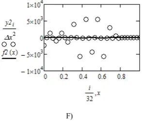
In Fig. 2D-2F are submitted the results of reconstruction of coefficients of Hermite quintic splines S5(x) under a
condition of zeroing of 50 wavelet-coefficients that are smaller 0.021 on the modulus. The attempt of zeroing of the following wavelet-coefficient D153= – 0.02347 that equals
A)
B)
C)
D)
E)
[image:8.595.360.507.78.203.2]F)
Figure 2. Diagrams of the wavelet-reconstruction of coefficients of Hermite quintic splines (A, B, C – for quintic function f (x) = x(x–2)(x–1)3,
its first and second derivatives; D, E, F – for function of Harten, its first and second derivatives).
5. Conclusion
It is simple to offer parallel realization of the algorithm, submitted in article, of wavelet-transformation of Hermite quintic splines, in which three direct courses of sweep method are carried out independently, and three inverses of courses are carried out with the maximal delay on two steps. Let's remind that the parallel algorithm of wavelet transformation of Hermite cubic splines provides the independent solutions of two three-diagonal systems. It would be interesting to find out, what is the degree of parallelism of wavelet transformation of Hermite septimus splines.
Acknowledgements
The reported study was partially supported by RFBR, research project No. 13-01-90900_mol_in_nr.
REFERENCES
[1] I. Daubechies. Ten Lectures on Wavelets, CBMS-NSF Reg. Conf. Ser. Appl. Math., Vol. 61, SIAM Ltd., Philadelphia, 1992.
[2] C. K. Chui. An Introduction to Wavelet Analysis, Academic Press Ltd., Boston, 1992.
[3] E. J. Stollnitz, T. D. DeRose, D. H. Salesin. Wavelets for Computer Graphics, Morgan Kaufmann Series, Elsevier Publ. Ltd., Amsterdam, 1996.
[4] V. Strela. Multiwavelets: Theory and Applications, Ph.D. Thesis in Mathematics, Cambridge University, Massachusetts, 1996.
[5] C. Heil, G. Strang, V. Strela. Approximation by translate of refinable functions, Numer. Math., Vol. 73, pp. 75-94, 1996. doi:10.1007/s002110050185
multiwavelets on the interval: cubic Hermite splines, Constr. Approx., Vol. 16, pp. 221-259, 2000.
doi:10.1007/s003659910010
[7] B. Han. Approximation properties and construction of
Hermite interpolants and biorthogonal multiwavelets, J. Approxim. Theory, Vol. 110, pp. 18-53, 2001.
doi:10.1006/jath.2000.3545
[8] R.-Q. Jia, S.-T. Liu. Wavelet bases of Hermite cubic splines on the interval, Advances Computational Mathematics, Vol. 25, pp. 23-39, 2006.
doi:10.1007/s10444-003-7609-5
[9] B. M. Shumilov, S. M. Matanov. Supercompact cubic
multiwavelets and algorithm with splitting, Proceedings of 2011 International conference on multimedia technology of
the IEEE, Hangzhou, China, 26-28 July 2011, Vol. 3, pp. 2636–2639, 2011.
doi:10.1109/ICMT.2011.6002586
[10] B. M. Shumilov. Cubic multiwavelets orthogonal to
polynomials and a splitting algorithm, Numerical Analysis and Applications, Vol. 6, Issue 3, pp. 247-259, 2013.
doi: 10.1134/S1995423913030087
[11] S. D. Conte, C. de Boor. Elementary Numerical Analysis: An Algorithmic Approach, Mcgraw-Hill College, 1980. – 3rd ed. [12] F. Arandiga, A. Baeza, R. Donat. Discrete multiresolution

![Table 1. Values of basic functions and their derivatives in points of an interval [0, 2]](https://thumb-us.123doks.com/thumbv2/123dok_us/8786698.907262/6.595.162.447.80.255/table-values-basic-functions-derivatives-points-interval.webp)