A Stochastic EM Algorithm for Progressively Censored Data Analysis

A Stochastic EM Algorithm for

Progressively Censored Data Analysis

Mimi ZHANG, Zhi-Sheng YE and Min XIE

Department of Systems Engineering & Engineering Management, City University of Hong

Kong

Abstract

Progressive censoring technique is useful in lifetime data analysis. Simple approaches to progressive data analysis are crucial for its widespread adoption by reliability engineers. This study develops an efficient yet easy-to-implement framework for analyzing progressively censored data by making use of the stochastic EM algorithm. Based on this framework, we develop specific stochastic EM procedures for several popular lifetime models. These procedures are shown to be very simple. We then demonstrate the applicability and efficiency of the stochastic EM algorithm by a fatigue life dataset with proper modification and by a progressively censored dataset from a life test on hard disk drives.

Key words: stochastic EM algorithm; progressively censored data; lifetime distribution

1

Introduction

tests. Generally speaking, a progressively censored sample of size 𝑛 consists of 𝑚 failures and 𝑛 − 𝑚 progressively censored observations. Censoring may happen right after a failure occurrence, i.e., remove 𝑅_𝑖 functioning units upon the 𝑖th failure, which is called progressive type II censoring. The progressive Type II censoring scheme has been applied to Burr-XII distributions (Wang and Cheng1), Weibull distributions (Pareek et al.2), Gaussian distributions (Balakrishnan et al.3), exponential distributions (Lee and Pan4) and log-logistic distributions (Balakrishnan and Saleh5), etc. Censoring can also happen in a random manner, which is common in medical studies, e.g., Davis and Feldstein6. Another example of random censoring is a life test conducted on a batch of raw hard disk drives (HDDs) in Seagate, a leading HDD company. Detailed description of the test will be introduced in Section 4. However, a problem faced by the HDD engineers is a lack of simple tools to analyze the data.

As noted by Ng et al.7, the complicated calculation of the likelihood function of progressively censored data when deriving the maximum likelihood estimates (MLEs) has greatly restricted the wide adoption of this scheme by reliability engineers. What engineers need is an efficient yet simple tool to compute the MLE. Employment of the standard or modified Newton–Raphson algorithm requires the Hessian matrix of the likelihood function, which differs from distributions to distributions and whose expression is most often quite complicated. An intuitive yet brute-force approach to maximizing the likelihood function of the progressively censored data is to directly apply some derivative-free algorithms, e.g., the ones reviewed by Kolda et al.8. However, as is well-known in the optimization literature, an algorithm has to visit every point in the feasible region in order to guarantee the global optimality, which is almost impossible when the parameter space is continuous. Moreover, most of these derivative-free algorithms will eventually converge to some local optimal points far away from the global optimum, if an educated starting point is not available.

based on complete data, which often has a simple closed form. However, with the increasing complexity of the progressively censored data and lifetime model, one of the biggest shortcomings of EM is that it is only a local optimization procedure and can easily get stuck in a saddle point. Moreover, when the E-step involves intricate or even infeasible computation, the EM paradigm is no longer directly applicable. A possible solution to overcoming the computational inefficiencies, i.e., the intractable E-step and the saddle point problem, is to invoke stochastic EM implementations such as the Monte Carlo EM algorithm (Wei and Tanner11). The Monte Carlo EM algorithm approximates the expectation in the E-Step by the Monte Carlo average. Therefore, the maximization of the averaged log-likelihood may be very complicated and thus more time-consuming, e.g., see Wang and Cheng1 for an application of the Monte Carlo EM algorithm to the Burr-XII distribution.

The stochastic EM (SEM) algorithm proposed by Celeux and Diebolt12 is also a stochastic version of the EM implementations as a way for executing the E-step by simulation. A very attractive merit of this algorithm is that it replaces the E-Step with an S-Step, which is very easy to implement whatever the underlying distribution and the missing data are. Compared with the Monte Carlo EM algorithm, the SEM algorithm completes the observed sample by replacing each missing datum by a value randomly drawn from the distribution conditional on results from the previous step. The M-step is thus a complete-data maximum likelihood estimation, which is often very easy to solve. The SEM algorithm has been shown to be computationally less burdensome and more appropriate than the EM algorithm in a lot of problems (Celeux and Diebolt12, Tregouet et al.13, Delignon et al.14, Cariou and Chehdi15). It is shown by Nielsen16 that the SEM algorithm always converges to some local optimum. Some applications of the SEM algorithm suggest that this algorithm tends to converge to the global optimum or a non-significant local optimum (Diebolt and Celeux17, Cariou and Chehdi15, Svensson and Sjöstedt-de Luna18).

from the previous SEM cycle, while the M-Step maximizes a complete sample likelihood function, which can be easily accomplished by most statistical software, e.g., Matlab, R, JMP, Minitab, SAS, SPSS, and S–PLUS. The procedure is thus very easy to implement yet efficient, which meets the needs of engineers. This framework is then applied to several common distributions, including the Weibull, lognormal, inverse Gaussian, and Birnbaum-Saunders distributions, etc. We only focus on point estimation. Confidence intervals for the parameters can be constructed based on the Hessian matrixes derived in the literature for each distribution, (Wang and Cheng1, Pareek et al.2, Balakrishnan et al.3, Balakrishnan and Saleh5).

The remainder of this paper is organized as follows. Section 2 develops the framework of progressively censored data analysis using the SEM algorithm. Section 3 elaborates on how this framework can be applied to a number of common distributions. In Section 3.5, a dataset from Birnbaum and Saunders19 and Ng et al.20, after proper modification, is fitted by the Birnbaum-Saunders distribution to demonstrate the simplicity of our method. We also apply the methodology to analyze a real dataset from a HDD test. Section 5 concludes the paper and points out possible topics for future research.

2

Analysis of Progressively Censored Data via SEM: A General

Framework

To simplify the notation, we consider data from a progressive type-II right censoring scheme, because of its popularity and its standards in notations. But we shall underscore that the framework applies to general progressively censored data, as will be demonstrated in Section 4.2. Under this scheme, 𝑛 ∈ ℕ identical units are placed on a life-test. Their lifetimes are described by independent and identically distributed random variables 𝑇₁, … , 𝑇_𝑛, each with probability density function (PDF) 𝑓(𝑡; Θ) and cumulative distribution function (CDF)

𝐹(𝑡; Θ), where Θ denotes the vector of model parameters. At the time of the first failure 𝑡₁,

𝑅₁ of the 𝑛 − 1 surviving units are randomly withdrawn from the experiment. 𝑅₂ of the

Type-II right censoring scheme with 𝑅𝑗 > 0 and ∑𝑚𝑗=1𝑅𝑗+ 𝑚 = 𝑛. The likelihood function based on the progressively censored data is

𝐿(Θ) = 𝑐 ∏ 𝑓(𝑡_𝑗; Θ)[1 − 𝐹(𝑡_𝑗; Θ)]𝑅𝑗

𝑚

𝑗=1

(1)

where 𝑐 = 𝑛(𝑛 − 𝑅₁− 1) … (𝑛 − 𝑅₁− 𝑅₂− ⋯ − 𝑅_𝑚−1− 𝑚 + 1). Equation (1) is generally difficult to optimize directly.

Denote the observed (ordered) failure data by 𝑻 = (𝑇_1:𝑚:𝑛, 𝑇_2:𝑚:𝑛, … , 𝑇_{𝑚:𝑚:𝑛}) and the unobserved censored data by 𝒁 = (𝒁₁, 𝒁₂, … , 𝒁_𝑚). 𝒁𝑗 (𝑗 = 1, … , 𝑚) is a 1 × 𝑅𝑗 random vector with 𝒁_𝑗 = (𝑍_𝑗1, 𝑍_𝑗2, … , 𝑍_𝑗𝑅𝑗) which represents the survival times of 𝑅𝑗 withdrawn units. The conditional distribution of the random variable 𝑍𝑗𝑙 (𝑙 = 1, … , 𝑅𝑗) given 𝑇𝑗:𝑚:𝑛= 𝑡𝑗

(𝑗 = 1, … , 𝑚) is given by (Ng et al.7)

𝐺_{𝑗(𝑧; Θ|𝑇𝑗:𝑚:𝑛} = 𝑡_𝑗) = 𝐹(𝑧; Θ)−𝐹(𝑡𝑗; Θ)

1−𝐹(𝑡𝑗; Θ) 𝑧 > 𝑡𝑗. (2)

The unobserved 𝒁 can be regarded as missing data. Given the complete data 𝑻 and 𝒁, the log-likelihood function of the complete sample can be specified as

𝑄(Θ) = ∑𝑚𝑗=1log 𝑓(𝑡𝑗; Θ)+ ∑𝑚𝑗=1∑𝑅_𝑙=1𝑗 log 𝑓(𝑧𝑗𝑙; Θ), (3)

The EM algorithm is an iterative algorithm. The E-step of the regular EM algorithm obtains the Q-function by taking the expectation of (3) with respect to the 𝒁 conditional on observed data 𝒁 and Θ(𝑘), the current value of Θ after k cycles of the EM algorithm. In view of the difficulty that the expectation is often very difficult, or even intractable to compute, the main idea of the SEM algorithm is to replace the E-step by a stochastic step where the missing data

S-Step. Given the current _ k _{, simulate} 𝑅

𝑗 independent values from the conditional distribution 𝐺_𝑗(𝑧; Θ(𝑘)|𝑇_{𝑗:𝑚:𝑛} = 𝑡_𝑗) respectively for 𝑗 = 1, … , 𝑚 to form a realization of 𝒁.

M-Step. Maximize the pseudo Q-function given (𝑻, 𝒁) to obtain Θ(𝑘+1).

The S-Step completes the data set in a very simple way, while the maximization in the M-Step deals with a complete sample. Hence the M-Step is easy to solve either explicitly or iteratively for most commonly-used distributions. Under mild regularity conditions, the sequence of

{Θ(𝑘)_{} starting from a specific Θ}(0) _{converges to a stationary distribution whose mean is a} consistent and asymptotically efficient estimator of parameters for the progressively censored data, i.e., the large sample variance-covariance matrix of the mean is exactly the Fisher information matrix (Diebolt and Celeux17, Diebolt and Ip21, Nielsen16, Svensson and Sjöstedt-de Luna18). It is easy to show that the regularity condition on smoothness of the underlying model is met for distributions discussed in Section 3. Therefore, we can run the SEM algorithm for a specific number of iterations, discard a few initial iterations for burn-in purpose, and average over Θ(𝑘) of the remaining iterations to obtain the MLEs. According to our experience, a burn-in period of 100 cycles is usually long enough under moderate censoring. A trace plot of the {Θ(𝑘)} sequence versus the cycles is also helpful for checking sufficiency of the burn-in period or for determining a more appropriate burn-in duration.

3

SEM Algorithms for Some Commonly Used Lifetime Distributions

To show the wide applicability of the framework developed in Section 2 and to elaborate on the flexibility of the SEM algorithm in handling progressively censored data, this section applied this framework to some common distributions used in lifetime data analysis in order.

3.1

Birnbaum-Saunders Lifetime Data

respective CDF and PDF of a two-parameter Birnbaum-Saunders random variable with a shape parameter 𝜇 and a scale parameter 𝜆 can be written as

𝐹(𝑡; 𝜇, 𝜆) = Φ {_𝜇1[(𝑡_𝜆)

1 2_{− (}𝜆

𝑡)

1

2_{]} , 𝑡 > 0}

,

𝑓(𝑡; 𝜇, 𝜆) = 1

2√2𝜋𝜇𝜆[( 𝜆 𝑡)

1 2

+ (𝜆_𝑡)

3 2

] × exp [−_2𝜇1₂(_𝜆𝑡+𝜆_𝑡− 2)] , 𝑡 > 0.

In the literature, Ng et al.20 have studied MLE of this distribution under type-II censoring by means of direct optimization of the likelihood function and the Monte Carlo EM algorithm. Their procedures tend to be very complicated due to the complex form of the likelihood function. On the contrary, the SEM algorithm is a handy gadget to handle this kind of censored data. Consider the progressively censored data (𝑻, 𝒁) generated from this distribution. Denoting Θ(𝑘)= (𝜇(𝑘), 𝜆(𝑘)) the value of Θ at the 𝑘th SEM cycle, the

(𝑘 + 1)st cycle proceeds as follows.

The S-Step

The conditional distribution function of the unobserved 𝑍𝑗𝑙 (𝑙 = 1, … , 𝑅𝑗) given 𝑇𝑗:𝑚:𝑛= 𝑡𝑗

(𝑗 = 1, … , 𝑚) is

𝐺_𝑗(𝑧; 𝜇, 𝜆|𝑇_{𝑗:𝑚:𝑛} = 𝑡_𝑗) =𝐹(𝑧; 𝜇,𝜆)−𝐹(𝑡𝑗; 𝜇,𝜆)

1−𝐹(𝑡_𝑗; 𝜇,𝜆) 𝑡 > 𝑡𝑗. (4) In other words, given 𝑇𝑗:𝑚:𝑛 = 𝑡𝑗, 𝑍𝑗𝑙 is a Birnbaum-Saunders variable left-truncated at 𝑡𝑗. Given (4), a random realization of 𝒁 is readily generated from 𝐺_𝑗(𝑧; 𝜇(𝑘), 𝜆(𝑘)|𝑇_{𝑗:𝑚:𝑛} = 𝑡_𝑗).

The M-Step

𝑄(𝜇, 𝜆) = −n log 2√2𝜋 − n log 𝜇 − n log 𝜆 + ∑ log [(𝜆 𝑡𝑖)

1 2

+ (𝜆 𝑡𝑖)

3 2

]

𝑚

𝑖=1

− ∑ 1 2𝜇2(

𝑡𝑖

𝜆 + 𝜆 𝑡_𝑖 − 2)

𝑚

𝑖=1

+ ∑ ∑ log [(𝜆 𝑧_𝑖𝑗)

1 2

+ (𝜆 𝑧_𝑖𝑗)

3 2 ] 𝑅𝑗 𝑗=1 𝑚 𝑖=1

− ∑ ∑ 1 2𝜇2(

𝑧𝑖𝑗

𝜆 + 𝜆 𝑧_𝑖𝑗 − 2)

𝑅𝑗

𝑗=1 𝑚

𝑖=1

.

To maximize this Q-function, we define the following function

𝐾(𝑥) = [_𝑛1(∑𝑚𝑖=1(𝑥 + 𝑡𝑖)−1+ ∑𝑚𝑖=1∑𝑅_𝑗=1𝑗 (𝑥 + 𝑧𝑖𝑗)−1)] −1

𝑥 ≥ 0,

where

𝑠 =_𝑛1(∑𝑚𝑖=1𝑡𝑖+ ∑𝑚𝑖=1∑𝑅_𝑗=1𝑗 𝑧𝑖𝑗) , 𝑟 = [1_𝑛(∑𝑚𝑖=1𝑡𝑖−1+ ∑𝑖=1𝑚 ∑_𝑗=1𝑅𝑗 𝑧𝑖𝑗−1)] −1

.

are the sample arithmetic and the sample harmonic means, respectively. From the results of complete sample MLE discussed by Birnbaum and Saunders19, we can see that the value of

𝜆(𝑘+1) _{is the unique positive root of the equation}

𝜆2_{− 𝜆[2𝑟 + 𝐾(𝜆)] + 𝑟[𝑠 + 𝐾(𝜆)] = 0.}

Once 𝜆(𝑘+1) is obtained, 𝜇(𝑘+1) can be derived explicitly as

𝜇(𝑘+1) _{= [} 𝑠 𝜆(𝑘+1)+

𝜆(𝑘+1) 𝑟 − 2]

1 2

.

Again, most statistical software provides packages that are able to do the complete sample estimation for the Birnbaum-Saunders distribution. Therefore, the M-step is indeed very easy to implement.

3.2

Gamma Lifetime Data

𝑓(𝑡; 𝜇, 𝜆) = 1 Γ(𝜇)

𝑡𝜇−1

𝜆𝜇 exp {−

𝑡

𝜆} , 𝑡 > 0,

where 𝜇 > 0 is a shape parameter and 𝜆 > 0 is a scale parameter. The CDF is

𝐹(𝑡; 𝜇, 𝜆) = 1

Γ(𝜇)∫ 𝑣𝜇−1𝑒−𝑣𝑑𝑣

𝑡/𝜆 0

=𝛾(𝜇, 𝑡/𝜆)

Γ(𝜇) , 𝑡 > 0,

where 𝛾(𝑎, 𝑏) is the lower incomplete gamma function given by

𝛾(𝑎, 𝑏) = ∫ 𝑣𝑏 𝑎−1_𝑒−𝑣_𝑑𝑣 0

.

Consider the progressively censored data (𝑻, 𝒁) generated from the above gamma distribution. Given the parameter values Θ(𝑘)= (𝜇(𝑘), 𝜆(𝑘)) obtained from the 𝑘th SEM cycle, The missing datum 𝑍𝑗𝑙 (𝑙 = 1, … , 𝑅𝑗) can be imputed from the following CDF

𝐺_𝑗(𝑧; 𝜇(𝑘)_{, 𝜆}(𝑘)_|𝑇

𝑗:𝑚:𝑛= 𝑡𝑗) =

𝛾(𝜇(𝑘)_{, 𝑧/𝜆}(𝑘)_{) − 𝛾(𝜇}(𝑘)_{, 𝑡}

𝑗/𝜆(𝑘))

Γ(𝜇(𝑘)_{) − 𝛾(𝜇}(𝑘)_{, 𝑡}

𝑗/𝜆(𝑘))

, 𝑡 > 𝑡_𝑗.

The pseudo Q-function based on data the imputed data is

𝑄(𝜇, 𝜆) = −𝑛 ln Γ(𝜇) − 𝑛𝜇 ln 𝜆 + (𝜇 − 1) ∑ ln 𝑡_𝑗

𝑚

𝑗=1

− ∑𝑡𝑗 𝜆

𝑚

𝑗=1

+ (𝜇 − 1) ∑ ∑ ln 𝑧_𝑗𝑙

𝑅𝑗

𝑙=1 𝑚

𝑗=1

− ∑ ∑𝑧𝑗𝑙 𝜆 𝑅𝑗 𝑙=1 𝑚 𝑗=1 .

The standard procedure to derive MLEs from this complete sample gamma Q-function is to first get 𝜇(𝑘+1) by solving

∑ ln 𝑡𝑗 𝑚

𝑗=1

+ ∑ ∑ ln 𝑧𝑗𝑙 𝑅𝑗

𝑙=1 𝑚

𝑗=1

+ 𝑛 ln 𝑛 + 𝑛 ln 𝜇(𝑘+1)_{− 𝑛𝛹(𝜇}(𝑘+1)₎

= 𝑛 ln (∑ 𝑡_𝑗

𝑚

𝑗=1

+ ∑ ∑ 𝑧_𝑗𝑙

𝑅𝑗

𝑙=1 𝑚

𝑗=1

)

𝜆(𝑘+1) ₌∑𝑚𝑗=1𝑡𝑗+∑𝑚𝑗=1∑𝑅𝑗𝑙=1𝑧𝑗𝑙

𝑛𝜇(𝑘+1) .

Remark: The above SEM procedure is also applicable to some variants of the gamma variable. For example, the inverse gamma distribution as a lifetime model has been suggested by Glen24. An inverse gamma random variable can be converted to a gamma variable by taking the reciprocal. Therefore, we can first take the reciprocal of the progressively censored data from an inverse gamma distribution, and then obtain MLEs of the parameters using the above procedure. Similarly, progressively censored data from the log-gamma distribution can be analyzed using the above procedure after an exponential transformation.

3.3

Inverse-Gaussian Lifetime Data

The inverse Gaussian distribution as a lifetime model has been promoted by many researchers (e.g., Chhikara and Folks23) due to its physical interpretation, i.e., the first passage time distribution of a Wiener process with a drift. This distribution has numerous good properties. Its PDF accommodates a variety of shapes, from highly skewed to almost normal; its failure rate function is unimodal with a limiting value greater than 0, providing a suitable choice for a lifetime model. See Chhikara and Folks23 for more details of this distribution. The respective PDF and CDF of an inverse Gaussian variable with the shape parameter 𝜇 and the mean 𝜆 are

𝑓(𝑡; 𝜇, 𝜆) = √_2𝜋𝑡𝜇3exp {

−𝜇(𝑡−𝜆)2

2𝜆2_𝑡 } , 𝑡 > 0;.

𝐹(𝑡; 𝜇, 𝜆) = Φ [√𝜇_𝑡(𝑡_𝜆− 1)] + exp (2𝜇_𝜆) Φ [−√𝜇_𝑡(_𝜆𝑡+ 1)] , 𝑡 > 0;

where Φ(∙) is the CDF of the standard normal distribution. Consider the progressively censored data (𝑻, 𝒁) generated from this distribution. If the missing data 𝒁 were known, MLE of the parameters based on (𝑻, 𝒁) can be specified as

λ̂ =∑ 𝑡𝑖

𝑚

𝑖=1 +∑𝑚𝑖=1∑𝑅𝑗𝑗=1𝑧𝑖𝑗

𝑛 , 𝜇̂

−1 ₌∑𝑚𝑖=1(𝑡𝑖−1−𝜆̂−1)+∑𝑖=1𝑚 ∑𝑅𝑗𝑗=1(𝑧𝑖𝑗−1−𝜆̂−1)

However, 𝒁 are indeed unknown. Under the SEM paradigm, they have to be imputed from the conditional distribution

𝐺_𝑗(𝑧; 𝜇, 𝜆|𝑇_{𝑗:𝑚:𝑛}= 𝑡_𝑗) = 𝐹(𝑧; 𝜇, 𝜆) − 𝐹(𝑡𝑗; 𝜇, 𝜆)

1 − 𝐹(𝑡_𝑗; 𝜇, 𝜆) 𝑡 > 𝑡𝑗

in the S-Step, after which the M-Step can be readily updated in terms of (5).

3.4

Lognormal Lifetime Data

The lognormal distribution is another commonly used lifetime model. Its PDF is given by

𝑓(𝑡; 𝜇, 𝜆) =_{𝑡√2𝜋𝜆}1 ₂exp {−(𝑙𝑛 𝑡−𝜇)_2𝜆2 2} (6)

In the presence of censoring data, the log-likelihood function does not have close form expression because of the survival function of the lognormal distribution involved (Bennett22). The EM algorithm for this distribution is thus preferable, and it has been developed by Ng et al.7. We will show that such data can also be easily handled by the SEM algorithm. Denoting

Θ(𝑘)_{= (𝜇}(𝑘)_{, 𝜆}(𝑘)_{) the value of Θ at the 𝑘th SEM cycle, the (𝑘 + 1)st step evolves as} follows.

S-Step

To impute the missing data, we need the conditional distribution of 𝑍𝑗𝑙 (𝑙 = 1, … , 𝑅𝑗), which is given by

𝐺_𝑗(𝑧; 𝜇, 𝜆|𝑇_{𝑗:𝑚:𝑛} = 𝑡_𝑗) =Φ (

ln 𝑧 − 𝜇

𝜆 ) − Φ ( 𝑡𝑗 − 𝜇

𝜆 ) 1 − Φ (𝑡𝑗− 𝜇_{𝜆 )}

𝑧 > 𝑡_𝑗.

A realization of the missing data 𝒁 can then be easily generated by imputing 𝑅𝑗 i.i.d. samples from 𝐺_𝑗(𝑧; 𝜇(𝑘), 𝜆(𝑘)|𝑇_{𝑗:𝑚:𝑛} = 𝑡_𝑗 ), 𝑗 = 1, … , 𝑚.

M-Step

𝜇(𝑘+1) ₌∑𝑚𝑖=1ln 𝑡𝑖+∑𝑚𝑖=1∑𝑅𝑗𝑗=1ln 𝑧𝑖𝑗

𝑛 ,

𝜆(𝑘+1) _{= √}∑ [ln 𝑡𝑖−𝜇(𝑘+1)]

2 𝑚

𝑖=1 +∑𝑚𝑖=1∑𝑅𝑗_𝑗=1[ln 𝑧𝑖𝑗−𝜇(𝑘+1)]2

𝑛

.

3.5

Weibull Lifetime Data

The Weibull distribution is one of the most widely used models in reliability and survival analysis. The respective PDF and CDF of this two-parameter model are

𝑓(𝑡; 𝜇, 𝜆) =𝜇_𝜆× (_𝜆𝑡)𝜇−1× exp {− (_𝜆𝑡)𝜇} , 𝑡 > 0, (7)

𝐹(𝑡; 𝜇, 𝜆) = 1 − exp {− (𝑡 𝜆)

𝜇

} , 𝑡 > 0,

where 𝜇 > 0 is a shape parameter, and 𝜆 > 0 is a scale parameter. Ng et al.7 has shown how to estimate the model parameters via the EM algorithm. Their method has to work on the log-lifetime that follows an extreme value distribution, and then transform the MLEs of the parameters in the extreme value distribution to the MLEs of the Weibull parameters. On the contrary, the SEM algorithm is able to avoid such transformation and work directly on the Weibull distribution, making the estimation more straightforward and simpler.

Consider the progressively censored data (𝑻, 𝒁) generated from the Weibull distribution (7). 𝑻 are the observed data while 𝒁 are considered as missing data. Given the complete data (𝑻, 𝒁), The log-likelihood function can be expressed as

𝑄(𝜇, 𝜆) = 𝑛(ln 𝜇 − ln 𝜆) + (𝜇 − 1) ∑𝑚𝑗=1(ln 𝑡𝑗− ln 𝜆)− ∑ ( 𝑡𝑗

𝜆) 𝜇 𝑚

𝑗=1

+(𝜇 − 1) ∑𝑚𝑗=1∑𝑅_𝑙=1𝑗 (ln 𝑧𝑗𝑙 − ln 𝜆)− ∑ ∑ ( 𝑧𝑗𝑙

𝜆) 𝜇 𝑅𝑗

𝑙=1 𝑚

𝑗=1 . (8)

The S-Step

To implement the S-step, the conditional CDF of 𝑍_𝑗𝑙 (𝑙 = 1, … , 𝑅_𝑗) given 𝑇_{𝑗:𝑚:𝑛} = 𝑡_𝑗

(𝑗 = 1, … , 𝑚) is needed, which is readily obtained as

𝐺_𝑗(𝑧; 𝜇, 𝜆|𝑇_{𝑗:𝑚:𝑛} = 𝑡_𝑗) = 1 − exp ((𝑡𝑗

𝜆) 𝜇

− (𝑧_𝜆) 𝜇) 𝑧 > 𝑡_𝑗.

Based on this conditional CDF, we can readily impute 𝒁𝑗, 𝑗 = 1, … , 𝑚, by generating 𝑅𝑗 i.i.d. samples from 𝐺_𝑗(𝑧; 𝜇(𝑘), 𝜆(𝑘)|𝑇_{𝑗:𝑚:𝑛}= 𝑡_𝑗). The imputed 𝒁𝑗 makes up a random realization of 𝒁. This random realization of 𝒁 in conjunction with the observed data is substituted into (8) to get the pseudo Q-function for the M-Step.

The M-Step

After attaining the pseudo Q-function (8) by making use of the imputed 𝒁 from the S-Step, the M-Step aims to obtaining Θ(𝑘+1) by maximizing this Q-function. The standard procedure to maximize this complete sample Weibull likelihood function is to first derive 𝜇(𝑘+1) by solving

∑𝑚𝑗=1𝑡𝑗𝜇×ln 𝑡𝑗+∑𝑚𝑗=1∑𝑅𝑗𝑙=1𝑧𝑗𝑙𝜇×ln 𝑧𝑗𝑙

∑𝑚𝑗=1𝑡𝑗𝜇+∑𝑚𝑗=1∑𝑅𝑗𝑙=1𝑧𝑗𝑙𝜇

−1_𝜇−1_𝑛(∑𝑚 ln 𝑡_𝑗

𝑗=1 + ∑𝑚𝑗=1∑𝑅_𝑙=1𝑗 ln 𝑧𝑗𝑙) = 0,

and then obtain 𝜆(𝑘+1) by making use of 𝜇(𝑘+1) as

𝜆(𝑘+1) _{= [}∑𝑚𝑗=1𝑡𝑗𝜇(𝑘+1)+∑𝑚𝑗=1∑𝑅𝑗𝑙=1𝑧𝑗𝑙𝜇(𝑘+1)

𝑛 ]

1/𝜇(𝑘+1) .

4

Two Illustrative Examples

4.1

The Birnbaum-Saunders Distribution for the Fatigue Life Data

Consider a dataset from Birnbaum and Saunders19 on the fatigue life of 6061-T6 aluminum coupons cut parallel to the direction of rolling and oscillated at 18 cycles per second, with a maximum stress per cycle at 31,000 psi. The original data were presented in Table 2 in Birnbaum and Saunders19. MLE of the Birnbaum-Saunders parameters based on this complete sample is

𝜇̂ = 0.170, 𝜆̂ = 131.8.

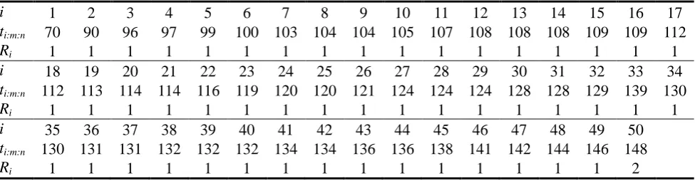
Ng et al.20 have used this dataset to demonstrate their inference procedure under type-II censoring. In this study, we use this dataset to demonstrate the applicability of the SEM algorithm for progressively censored data from the Birnbaum-Saunders distribution. Based on the original data, we randomly generate a progressively censored dataset with 𝑚 = 50 and a progressively censored scheme 𝑅_𝑖 = 1 for 𝑖 < 50 and 𝑅₅₀= 2. The generated data are displayed in Table 1.

We apply the SEM procedure developed in Section 3.1 to analyze this progressively censored dataset. The initial value of 𝜇 and 𝜆 for the algorithm are set as 𝜇(0)= 1 and 𝜆(0)= 100, which is far away from the MLE. The number SEM cycles is set as 1100. The first 100 cycles are used as burn-in period, while the additional 1000 cycles are averaged to estimate model parameters.

Figure 1 shows the trace plots of these two parameters versus the SEM cycles. The values of the parameters oscillate with the SEM cycles around the bold horizontal lines in Figure 1, but do not show any uptrend or downtrend. This suggests that the Markov Chain {Θ(𝑘)} has converged to a stationary distribution. The average of the sequence {Θ(𝑘)} would be sufficient to approximate the MLE, which is

𝜇̂ = 0.1735, 𝜆̂ = 131.2.

derivative-free algorithms reviewed in Kolda et al.8. The brute-force maximization yields an estimate of

𝜇̂ = 0.1739, 𝜆̂ = 131.2,

which is very close to the results given by the SEM algorithm. The difference may be due to some simulation variations. This similarity implies the efficacy of the SEM algorithm in dealing with the censored data.

Given the complete sample with sample size 𝑛 = 101, an extensive simulation study is conducted to investigate the impact of the sampling scheme, i.e. the failure number 𝑚 and the combination of withdrawn numbers {𝑅₁, 𝑅₂, … , 𝑅_𝑚}, on the performance of the SEM algorithm. The progressively Type-II censored dataset is generated randomly, that is, the withdrawn number 𝑅_𝑖 at the 𝑖th failure is randomly simulated under the constraint ∑𝑚_𝑖=1𝑅_𝑖 =

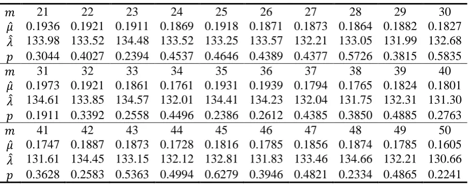
𝑛 − 𝑚. For each value of 𝑚, we randomly generate a progressively Type-II censored dataset and, using the SEM algorithm, we obtain an estimate vector of (𝜇, 𝜆), denoted as (𝜇̂, 𝜆̂). The Kolmogorov-Smirnov test (K-S test) is served as a goodness-of-fit test (compare the fitted distribution to the original complete data). By ranging 𝑚 from 21 to 50, the results are given in Table 2. In Table 2, the notation 𝑝 represents the 𝑝-value of the Kolmogorov-Smirnov test.

Form the 𝑝-value we can see that the increase of the failure number 𝑚 does not necessarily guarantee the improvement in the performance of the SEM algorithm. This result may seem counterintuitive in the sense that one would typically expect, with the failure number increasing, the 𝑝-value of the K-S test should increase. However, the fluctuating 𝑝-values can be explained as follows: for predetermined sample size 𝑛 and failure number 𝑚, the combination {𝑅₁, 𝑅₂, … , 𝑅_𝑚} has a considerable influence on the SEM algorithm. We repeat the preceding procedure for 20 times and plot the 𝑝 values in Figure 2. The increasing trend in Figure 2 indicates that, with the failure number increasing, the SEM algorithm will more fit the data.

4.2

The Lognormal Distribution for the HDD Failure Data

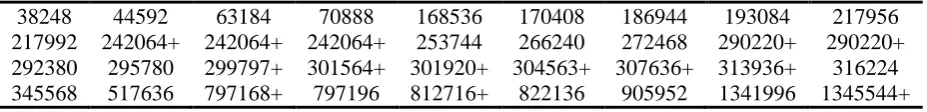
failures reveals that most failures attribute to particles accumulated in the disks. Therefore, the life test was conducted by injecting particles into 36 raw disks for a certain duration, during which the cumulative particle counts to failure for the failed disks were recorded. After the test, some units were still working, and their cumulative particle counts to failure data were censored. Due to the unstable injection rate for each unit, the censored cumulative particle counts for these units were different. Therefore, the data can be regarded as progressively censored. The data are shown in Table 3.

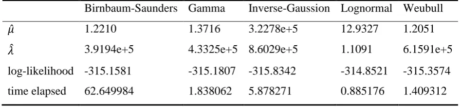
HDD engineers demand a convenient method that can effectively analyze the data. The SEM algorithm is thus favorable. We try all the distributions presented in Section 3 on this data set, and the results are listed in Table 4. The MLEs, which are obtained based on the exactly observed failure data, are set as the initial values of 𝜇 and 𝜆 in the SEM algorithm. As with the previous example, the number of SEM cycles is set as 1100, while the first 100 cycles are used for burn-in. Obviously, based on the value of the log-likelihood, the lognormal distribution is well-fit to the data. For each distribution, we also record the time the SEM algorithm consumes. All computations were coded in MATLAB (MathWorks, R2011b) on an Intel Core 2 6420 (Intel), 2.13 GHz PC with 2 GB RAM. As can be seen, the Birnbaum-Saunders distribution and the Inverse-Gaussion distribution take much more time than the other three distributions. This is rooted in the way we impute the missing data: To generate a sample from 𝐹_𝑗(𝑍_𝑗𝑙 ; Θ) in (2), we generate samples from 𝐹(𝑡; Θ) until we get the first one greater than 𝑡𝑗; see the appendix. If we use built-in random number generator, as in the other three cases, the algorithm is indeed very fast.

Therefore, the Lognormal distribution can be served as the underlying distribution, and the estimates for 𝜇 and 𝜆 are, respectively 𝜇̂ = 12.9327 and 𝜆̂ = 1.1091. The evolution paths of the parameters in the algorithm are depicted in Figure 3. As can be seen from this figure, no obvious trend is detected for the {Θ(𝑘)} sequence. By using the estimates from the SEM algorithm as a starting point, we numerically maximize the likelihood function by some optimization algorithms. The MLEs are

𝜇̂ = 12.920, 𝜆̂ = 1.084,

5

Conclusions

This study has developed a generic framework for analyzing the progressively censored data by using the stochastic EM algorithm. The algorithm iteratively implements the S-Step by drawing a sample from the conditional distribution of the missing data based on the parameter values from the previous step, while the M-Step is a complete sample likelihood maximization. Both steps can be easily implemented by making use of distribution packages provided by most statistical software. In addition, the stochastic nature enables the SEM algorithm to avoid getting stuck at a saddle point of the likelihood function, which is a headache faced by the traditional EM algorithm, and the Newton–Raphson method. In view of the fact that progressively censored data are common in real applications and that engineers prefer handy tools for the analysis, our framework is potentially very useful. We then presented a real dataset from a life test on 36 HDDs. The data were progressively censored, and the SEM algorithm was shown to be capable to effectively estimate the parameters with a short runtime.

In Section 4 we investigate the impact of the sampling scheme on the performance of the SEM algorithm. The results show that, with the failure number 𝑚 increasing, the 𝑝-value of the K-S test increases, i.e., the performance improves. However, for fixed sample size 𝑛 and failure number 𝑚, the combination of withdrawn numbers {𝑅₁, 𝑅₂, … , 𝑅_𝑚} is of great influence on the SEM algorithm. Future research can be done in determining the optimal sampling scheme. Also, future research can be done in studying whether the number of burn-in iterations depends on specific distributions and/or on initial parameter settings. This will help the practitioners to choose a favorable sampling scheme and appropriate number of cycles in their domain problems.

Appendix

The standard method is to use the fact that 𝐹_𝑗(𝑍_𝑗𝑙 ; Θ) follows a standard uniform distribution, i.e., 𝒰 = 𝐹_𝑗(𝑍_𝑗𝑙 ; Θ)~𝑈(0, 1). By using (2), we can see that

𝒰[1 − 𝐹(𝑡_𝑗; Θ)] + 𝐹(𝑡_𝑗; Θ) = 𝐹(𝑍_𝑗𝑙 ; Θ)

Therefore, we can first generate a random realization of 𝒰, say, 𝑢, and then obtain realization of 𝑍𝑗𝑙 as

𝑧_𝑗𝑙 = 𝐹−1_{(𝑢 + (1 − 𝑢)𝐹(𝑡}

𝑗; Θ) ; Θ), (9)

where 𝐹−1(∙) is the inverse function of 𝐹(∙). For example if 𝐹(∙) if the Weibull CDF, (9) can be explicitly written as

𝑧_𝑗𝑙 = 𝜆[(𝑡_𝑗/𝜆)𝜇_{− ln(1 − 𝑢)]}1/𝜇_,

However, close-form expressions of (9) for some distributions do not exist, e.g., the lognormal distribution and the gamma distribution. Luckily, most statistical software provides packages that can directly compute 𝐹−1(∙) for most distributions. This greatly simplifies the problem.

Another way to generate a sample from 𝐹_𝑗(𝑍_𝑗𝑙 ; Θ) in (2) is to generate samples from

𝐹(𝑡; Θ) until we get the first one greater than 𝑡𝑗. This method is somewhat brute-force. However, it is much easier to implement. In addition, almost all statistical software has random number generators for most common distributions, e.g., the ones discussed in Section 3.

References

1. Wang FK, Cheng YF. EM algorithm for estimating the Burr XII parameters with multiple censored data. Quality and Reliability Engineering International 2010; 26:

615-630.

3. Balakrishnan N, Kannan N, Lin CT, Ng HKT. Point and interval estimation for Gaussian distribution, based on progressively Type-II censored samples. IEEE Transactions on Reliability 2003; 52: 90-95.

4. Lee J, Pan R. Bayesian analysis of step-stress accelerated life test with exponential distribution. Quality and Reliability Engineering International 2012; 28: 353-361. 5. Balakrishnan N, Saleh HM. Relations for moments of progressively type-II censored

order statistics from log-logistic distribution with applications to inference. Communications in Statistics-Theory and Methods 2012; 41: 880-906.

6. Davis HT, Feldstein ML. The generalized Pareto law as a model for progressively censored survival data. Biometrika 1979; 66: 299-306.

7. Ng HKT, Chan PS, Balakrishnan N. Estimation of parameters from progressively censored data using EM algorithm. Computational Statistics & Data Analysis 2002; 39:

371-386.

8. Kolda TG, Lewis RM, Torczon V. Optimization by direct search: New perspectives on some classical and modern methods. SIAM Review 2003; 45: 385-482.

9. Lin CT, Wu SJS, Balakrishnan N. Inference for log-gamma distribution based on progressively type-II censored data. Communications in Statistics-Theory and Methods 2006; 35: 1271-1292.

10.Pradhan B, Kundu D. On progressively censored generalized exponential distribution. Test 2009; 18: 497-515.

11.Wei GCG, Tanner MA. A Monte Carlo implementation of the EM algorithm and the poor man's data augmentation algorithms. Journal of the American Statistical Association 1990; 85: 699-704.

12.Celeux G, Diebolt J. The SEM algorithm: a probabilistic teacher algorithm derived from the EM algorithm for the mixture problem. Computational Statistics Quarterly 1985; 2: 73-82.

13.Tregouet DA, Escolano S, Tiret L, Mallet A, Golmard JL. A new algorithm for haplotype-based association analysis: the Stochastic-EM algorithm. Annals of human genetics 2004; 68: 165-177.

14.Delignon Y, Marzouki A, Pieczynski W. Estimation of generalized mixtures and its application in image segmentation. IEEE Transactions on Image Processing 1997; 6:

15.Cariou C, Chehdi K. Unsupervised texture segmentation/classification using 2-D autoregressive modeling and the stochastic expectation-maximization algorithm. Pattern Recognition Letters 2008; 29: 905-917.

16.Nielsen FS. The stochastic EM algorithm: estimation and asymptotic results. Bernoulli 2000; 6: 457-489.

17.Diebolt J, Celeux G. Asymptotic properties of a stochastic EM algorithm for estimating mixing proportions. Stochastic Models 1993; 9: 599-613.

18.Svensson I, Sjöstedt-de Luna S. Asymptotic properties of a stochastic EM algorithm for mixtures with censored data. Journal of Statistical Planning and Inference 2010; 140:

111-127.

19.Birnbaum ZW, Saunders SC. Estimation for a family of life distributions with applications to fatigue. Journal of Applied Probability 1969; 6: 328-347.

20.Ng HKT, Kundu D, Balakrishnan N. Point and interval estimation for the two-parameter Birnbaum–Saunders distribution based on Type-II censored samples. Computational Statistics & Data Analysis 2006; 50: 3222-3242.

21.Diebolt J, Ip EHS. Stochastic EM: Method and application, in Markov chain Monte Carlo in practice, Chapman & Hall/CRC, 1996; 259-273.

22.Bennett S. Log-logistic regression models for survival data. Applied Statistics 1983; 32:

165-171.

23.Chhikara RS, Folks JL. The inverse Gaussian distribution as a lifetime model. Technometrics 1977; 19: 461-468.

Table 1. A progressively censored dataset generated from the original fatigue life data presented in Birnbaum and Saunders19 and Ng et al.20.

i 1 2 3 4 5 6 7 8 9 10 11 12 13 14 15 16 17

ti:m:n 70 90 96 97 99 100 103 104 104 105 107 108 108 108 109 109 112

Ri 1 1 1 1 1 1 1 1 1 1 1 1 1 1 1 1 1 i 18 19 20 21 22 23 24 25 26 27 28 29 30 31 32 33 34

ti:m:n 112 113 114 114 116 119 120 120 121 124 124 124 128 128 129 139 130

Ri 1 1 1 1 1 1 1 1 1 1 1 1 1 1 1 1 1 i 35 36 37 38 39 40 41 42 43 44 45 46 47 48 49 50

ti:m:n 130 131 131 132 132 132 134 134 136 136 138 141 142 144 146 148

Table 2. Estimated parameter values and 𝑝-value with changing 𝑚.

𝑚 21 22 23 24 25 26 27 28 29 30

𝜇̂ 0.1936 0.1921 0.1911 0.1869 0.1918 0.1871 0.1873 0.1864 0.1882 0.1827

𝜆̂ 133.98 133.52 134.48 133.52 133.25 133.57 132.21 133.05 131.99 132.68

𝑝 0.3044 0.4027 0.2394 0.4537 0.4646 0.4389 0.4377 0.5726 0.3815 0.5835

𝑚 31 32 33 34 35 36 37 38 39 40

𝜇̂ 0.1973 0.1921 0.1861 0.1761 0.1931 0.1939 0.1794 0.1765 0.1824 0.1801

𝜆̂ 134.61 133.85 134.57 132.01 134.41 134.23 132.04 131.75 132.31 131.30

𝑝 0.1911 0.3392 0.2558 0.4496 0.2386 0.2612 0.4385 0.3850 0.4885 0.2763

𝑚 41 42 43 44 45 46 47 48 49 50

𝜇̂ 0.1747 0.1887 0.1873 0.1728 0.1816 0.1785 0.1856 0.1874 0.1785 0.1605

𝜆̂ 131.61 134.45 133.15 132.12 132.81 131.83 133.46 134.66 132.21 130.66

Table 3. Progressively censored data of 36 HDDs based on cumulative particle counts: Censoring is indicated by +.

Table 4. Estimated parameter values and the likelihood result.

Birnbaum-Saunders Gamma Inverse-Gaussion Lognormal Weubull

𝜇̂ 1.2210 1.3716 3.2278e+5 12.9327 1.2051

𝜆̂ 3.9194e+5 4.3325e+5 8.6029e+5 1.1091 6.1591e+5