Experimental Studies on Dynamics Performance of Lateral and Longitudinal
Control for Autonomous Vehicle Using Image Processing
Khalid Isa
Department of Computer Engineering
Faculty of Electrical and Electronic Engineering
Universiti Tun Hussein Onn Malaysia
P.O Box 101, 86400 Parit Raja, Batu Pahat, Johor, Malaysia
[email protected]
Abstract
This paper presents a simulation of vehicle driving control system in terms of lateral and longitudinal control using image processing. The main contribution of this study is it contributes an algorithm of vehicle lane detection and tracking which based on colour cue segmentation, Canny edge detection and Hough transform. The algorithm gave good result in detecting straight and smooth curvature lane on highway even the lane was affected by shadow. Then by combining and processing the result of lane detection process with vehicle dynamics model, this system will produce the dynamics performance of vehicle driving control. This simulation system was divided into four subsystems: sensor, image processing, controller and vehicle. All the methods have been tested on video data and the experimental results have demonstrated a fast and robust system.
1. Introduction
The main objective of this system is to develop the simulation for analysing dynamics performance of lateral and longitudinal control for autonomous vehicle using image processing. Therefore, the simulation determines the steering command for the vehicle lateral control by processing, analysing, and detecting the lane on highway. This means, the lane detection process will produce the lane angle, and this angle was directly used as steering command. Then, by combining the steering command and others vehicle dynamics parameters such as the vehicle mass, and vehicle velocity, the vehicle’s dynamics performance can be determined by this system.
Previously, many lanes or road boundary detection algorithms have been developed. LOIS [1] system used a deformable template approach to find the best fit of road model whether it straight or curve. The research
groups of the University Der Bundeswehr [2] and Daimler-Benz [3] base their road detection functionality on a specific road model: lane markings are modelled as clothoids. This model has the advantage that the knowledge of only two parameters allows the full localization of lane markings and the computation of other parameters like the lateral offset within the lane, the lateral speed with respect to the lane and the steering angle. The approach in [4] is an evolutionary approach of lane markings detection. It used collaborative autonomous agents to identify the lane markings in road images.
Several aspects of designing control system for a vehicle have been examined extensively in the past, both in the physics literature [5] as well as in control theoretic studies. The control problem in a dynamic setting, using measurement ahead of the vehicle, has been explored by [6], who proposed a constant control law proportional to the offset from the centreline at a look-ahead distance. Ackermann et al [7], proposed a linear and non-linear controller design for robust steering. Taylor et al [8] considered the problem of controlling a motor vehicle based on the information obtained from conventional cameras mounted onboard. Ma, Kosecka and Sastry [9] looked at the problem of guiding a nonholonomic robot along a path based on visual input.
2. Problem Formulation
The following subsection presents the basic system design and the techniques.
2.1 System Design
System design for autonomous vehicle is depending on number of tasks that can be performed by the vehicle. Since the experiment only using one video camera as a sensor, so this paper only presented the lane detection task along with dynamics and control of
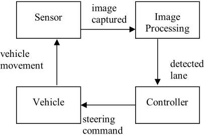
the vehicle. Figure 1 presents general flow of the system. The figure was consists into four subsystems: sensor (video camera), image processing, controller, and vehicle.
Figure 1: Four subsystems of vision-based autonomous vehicle driving control system
2.2. Sensor
This system used a single video camera as a sensor. A single colour video camera was mounted inside the vehicle behind the windshield along the central line. It takes the images of the environment in front of the vehicle, including the road, vehicles on the road, traffic signs on the roadside, and sometimes, incident objects on the road. The video camera saved the video image in AVI file format. Then the video file is transferred to the computer and then it captured the images 15 frames per second, and save it in the computer memory. The image processing subsystem takes image from the memory and start processing the image to detect the desired lane.
2.3. Image Processing and Analysis for Predicting and Detecting Vehicle Lane
In the lane detection process of this system, road area segmentation and shadow removal was handling using colour cues. Then it finds the best linear fits to the left and right lane markers over a certain look-ahead range through a variant of the Hough transform. From these measurements we can compute and estimate for the lateral position and orientation of the vehicle with respect to the roadway at a particular look-ahead distance.
2.3.1. Colour Cue Segmentation. The segmentation of the images is a crucial part for the analysis of the driving scenes. In this system, it used colour cue as the measure of segmentation. It will be shown as a colour-based visual module providing relevant information for
the localization of the visible road area, independent with the presence of lane boundary markings and different lighting conditions.
In the road image, road area has such characteristics as follows; most portions in lower part of the image are considered as the road area and road areas have quasi-uniform colour. Resulting from the observation that the road areas are generally grey surfaces placed into more coloured environment. To have a better control over variations in pixels values for the same colour and to remove the shadows, the RGB colour space must be converted to the HSV (hue, saturation, and value) space.
2.3.2. Extraction and Detection of Vehicle Lane Edges Using Canny Edge Detector. The purpose of edge detection process is to extract the lane edges by using edge detection operator or edge detector. The operator will locate the position of pixels where the significant pixels exist. The edges will be represents as white and non-edges will be black.
We used Canny edge detector to locate the position of pixels where significant edges exist. By applying the Canny edge detector to a road image, two images that denote the edges pixels and the orientation of gradient can be obtained. The Canny’s criterion for good detection is low probability of not marking real edge points, and falsely marking non-edge points. This is achieved by using the following equation
∫
∫
− −
−
=
ww o w
w
dx
x
f
n
dx
x
f
x
G
SNR
)
(
)
(
)
(
2
(1)
f is the filter, G is the edge signal, denominator is the root-mean-squared(RMS) response to noise n(x) only. Besides, Canny’s good localization criterion is close to centre of the true edge. Below is the equation to measure the localization. It used reciprocal of RMS distance of the marked edge from the centre of the true edge.
Localization =
∫
∫
−
−
=
ww ,
, ,
(x)dx
f
n
(x)dx
x)f
(
G
]
E[x
20 2
0
1
(2)
2.3.3. Features Isolation and Approximation of Vehicle Lane Using Hough Transform. Hough
Sensor Image
Processing
Controller Vehicle
image captured
detected lane
steering command vehicle
transform is used to combine edges into lines, where a sequence of edge pixels in a line indicates that a real edge exists. By using the edge data of the road image, Hough transform will detect the lane boundary on the image. The key idea is to map a lines detection problem into a simple peak detection problem in the space of the parameters of the line. Although there are may be curves in the road geometry, straight-line will still be a fairly good approximation of lanes, especially within the reasonable range for vehicle safety because the curve is normally long and smooth.
Firstly, find all of the desired feature points in the image. Second, for each feature point, find possibility i
lines in the accumulator that passes through the feature point. Then, increment that position in the accumulator. After that, find local maximum in the accumulator. Lastly, if desired, map each maximum in the accumulator back to image space. After the coordinates of the lane line in the accumulator space have been identified, we remapped the line coordinates of the lane to the image space, so the lane can be highlighted.
2.3.4. Lane Tracking. Basically, since the capturing rate is 15 frames per second, the difference between images in the sequence will be very small. So, we do not need to process each entire image in terms of lane tracking. From the previous lane position, we can have a very good estimate of lane position in the current frame. Therefore, in the Hough transformation, the angle,θ, can be restricted by the estimated range from previous frames. This will improve the computational speed and the accuracy of detection. In each second, the first several image frames will be processed by the lane detection algorithm, and provide a good estimate of lane tracking for the next frames.
2.4. Vehicle Controller
In this system, we used feedback 2WS controller. Peng at el [10] had validated this, where the error signal was actually previewed slightly. As mentioned before, the vehicle controller requires a model of vehicle’s behaviour whether dynamics or kinematics model of vehicle. Therefore, in this system the controller based on the mathematical model of four wheels vehicle dynamics. In this system, longitudinal control and lateral control were focused.
2.4.1. Lateral Control. The lateral controller purpose is to follow the desired path. It only needs to know the car’s location with respect to the desired path. The lateral controller determined the steering angle based on the desired lane of the road. This steering angle
maintains the vehicle in a desired position on the road. Here, the idea is that the vehicle has some desired path to follow. Sensors on the vehicle detected the location of the desired path.
Steering angle δ =| θ1+θ2 -180° | (3)
The first step to understanding lateral control is to analyze the low speed turning behaviour. At low speed the tires need not develop lateral forces. They roll with no slip angle, and the vehicle must negotiate a turn. But at high speed the tires develop lateral forces, so the lateral acceleration presented. In lateral controller, lateral force, denoted by Fc, is called the cornering force when the chamber angle is zero. At a given tire load, the cornering force grows with slip angle. At low slip angle (5 degrees and less) the relationship is close to linear.
α
αC
F
c=
(4)The steady state cornering equations are derived from the application of Newton’s second law. For a vehicle-travelling forward with a speed of V, the sum of the forces in the lateral direction is:
∑
F
=
F
+
F
=
MV
2/
2
cr cf
c (5)
with the required lateral forces known, the slip angles at the front and rear wheels are also established.
)
/
(
/
L
V
2R
Mb
F
cr=
(6)L
c
W
W
f=
.
/
(7)L
Mgb
W
r=
/
(8))
/(
2
C
gR
V
W
f ff α
α
=
(9))
/(
2
C
gR
V
W
r rr α
α
=
(10)2.4.2. Longitudinal Control. This controller just depends on the longitudinal dynamics of vehicle. The behaviour of vehicle when driving straight ahead or at very small lateral acceleration values is defined as the longitudinal dynamics. From the longitudinal dynamics the calculation and evaluation of acceleration, braking and speed can be accomplished. Vehicle longitudinal dynamics was determined by forming Newton’s law by using the following equations:
s l
f r
x
U
U
W
G
υ
ma
=
+
−
−
⋅
sin
(11)s z
f
r
P
W
G
P
cos
υ
(
)
(
)
(
f r)
ysf f f r r r r r f f
MW
h
U
U
e
l
P
e
l
P
J
J
+
⋅
+
−
−
−
−
⋅
=
Ω
+
Ω
(13)
From these equations with equal rolling resistance coefficients for all wheels an equation for the longitudinal motion could be derived.
An equation for braking performance can be obtained from Newton’s second law. The sum of the external forces acting on a body in a given direction is equal to the product of its mass and the acceleration in that direction. Relating this law to straight-line vehicle braking, the significant factors are shown in following equation.
δ
δ
cos
sin
)
/
(
r a
xr xf x x
f
W
D
F
F
D
g
w
Ma
F
+
+
+
+
=
=
=
∑
(14)If braking forces are held constant and the vehicle velocity effects on aerodynamic drag and rolling resistance are neglected, the time for a vehicle velocity change can be derived from Newton’s second law. This is shown on following equation.
(
f)
xt
V
V
F
M
t
=
0−
(15)3. Problem Solution
This system was programmed using MATLAB 6.5 language. The initial experiments used real time data of image sequence taken from Malaysia highway. For experimental test, we used six different video scenes on highway. Each video consists hundred of frames. Since the processing of this system is based on video sensor, so we assumed in the first frame of the video, the vehicle is driving at certain velocity, at the last frame the vehicle is stop moving. This means that the vehicle is braking, and then the vehicle velocity changed. So, we calculated the brake forces, velocity and acceleration of the vehicle and this system shows the graphs.
[image:4.612.356.519.70.214.2]The following figures show the results of lane detection process using image processing techniques.
[image:4.612.351.522.246.402.2]Figure 2: Original image of frame one in RGB colour space
Figure 3: Hough transform accumulator to estimate lines coordinate of the lane
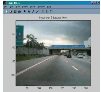
Figure 4: Original image with detected lane
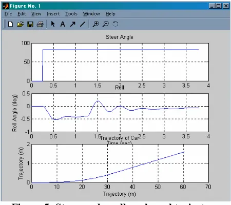
[image:4.612.351.520.434.588.2]Figure 5: Steer angle, roll angle and trajectory
[image:5.612.67.292.82.282.2]The simulation shows that the steering angle for the vehicle is 82 degrees and the roll angle after 1.25 seconds is getting smaller, which is approximate to 0 degree. This is because at 1.25 seconds the vehicle having brake forces until it stop moving. The vehicle trajectory in this situation reached 60 meter.
Figure 6: Velocity and longitudinal acceleration, lateral acceleration, yaw angle and sideslip angle
[image:5.612.66.289.384.575.2]The velocity graphs shows that the starting vehicle velocity is 26 m/sec and it getting slower because the vehicle experienced brake forces. When the velocity is slower, the longitudinal acceleration decreased. In the lateral acceleration graph, it shows that the acceleration in braking situation is much lower than normal situation.
Figure 7: Brake forces, normal forces and lateral forces
The brake forces graph shows that the rear tyres experienced heavy brake forces than front tyres. This is because the modelled vehicle in this system used front-wheel brake system. Therefore, most of the brake forces for the front tyres came from the braking system component, which was not totally from tyre-to-road interface forces. On the other hand, rear tyres experienced brake forces from tyre-to-road interface forces, which it provides tyre-to-road coefficient of friction.
From the normal forces graph, it shows that the front tyres experienced heavy normal forces than rear tyres. Logically, this is because the vehicle engine is in the front side. Therefore, normal load on front side of vehicle is heavier than rear side. For the lateral forces, the front tyres experienced heavy lateral forces than rear tyres because we used front-wheel-drive system for the vehicle. Theoretically, in front-wheel-drive vehicle, front tyres will experiences more lateral forces than rear tyres. This is because we used front wheels to drive the vehicle.
4. Conclusion
detection algorithm, a colour cue was used to conduct image segmentation. Then, Canny edge detection was used to extract the lane edges. After that, Hough transformation was used to detect the lanes and determined the look-ahead distance and the lanes angle. This method has been tested on video data, and the experimental results have demonstrated a fast and robust system.
This system used dynamics model to create more precise control algorithm. Then, the feedback controller was used to determine the lateral and longitudinal control of the vehicle. The implementation of dynamics model makes this system provides the dynamics performance of the vehicle such as vehicle velocity, acceleration, and vehicle forces. Besides, the implementation on non-linear tyres model provides the performance on each wheel. This system was applied and tested on high and low vehicle speed. Since, this system used dynamics model of the vehicle, therefore comparing with [11] and [12]; the results of this simulation showed that dynamics model approach gave highly accurate portrayal of the vehicle’s behaviour and the controllers designed with this approach are robust to those dynamics.
5. References
[1] Kreucher C., Lakshmanan S. and Kluge K., “A Driver Warning System Based on the LOIS Lane Detection Algorithm”. Proceeding of IEEE International Conference on Intelligent Vehicles, 1998, pp.17-22.
[2] U. Franke, D. Gavrilla, S. Gorzig, F. Lindner, F. Paetzold, C. Wohler, Autonomous Driving Goes Downtown, Proceedings of IEEE Intelligent Vehicle Symposium ’98, Stuttgart, Germany, October 1998, pp. 40-48.
[3] M. Lutzeler, E.D. Dickmanns, Road Recognition with MarVEye, Proceeedings of the IEEE Intelligents Vehicle Symposium ’98, Stuttgart, Germany, October 1998, pp 341-346.
[4] M. Bertozzi, A. Broggi, A. Fascioli, A. Tibaldi, “An Evolutionary Approach to Lane Markings Detection in Road Environments”, University De Parma, Italy, 2002.
[5] M.F. Land and D.N. Lee. “Where we look when we steer?”. Nature, vol 369, June 1994, pp 30.
[6] U. Ozguner, K.A. Unyelioglu, and C. Hatipoglu. “An analytical study of vehicle steering control”. In Proceedings of the 4th IEEE Conference on Control Applications, 1995,
pp 125-130.
[7] Ackermann, Juergen. Guldner, Juergen. Sienel, Wolfgang. Steinhauser, Reinhold. Utkin, Vadim I. “Linear and nonlinear controller design for robust automatic steering”. IEEE Transactions on Control Systems Technology. vol 3 no 1 Mar 1995, pp. 132-142.
[8] C. J. Taylor, J. Košecká, R. Blasi, and J. Malik, “A Comparative Study of Vision-based Lateral Control Strategies for Autonomous Highway Driving,” The Int. J. Robot. Research, vol. 18, no. 5, 1999, pp. 42-453.
[9] Y. Ma, J. Košecká, and S. Sastry, “Vision guided
navigation for nonholonomic mobile robot”. IEEE Trans.Robot. Automation., vol. 15, no. 3, June 1999, pp. 521-536.
[10] Peng, Huei, Webin Zhang, Masayoshi Tomizuka, and Steven Shladover. “A Reusability Study of Vehicle Lateral Control System”, Vehicle System Dynamics, no 28, 1994, pp 259-278.
[11] P. Mellodge, “Feedback Control for a Path Following Robotic Car”, Master Thesis, Virginia Polytechnic Institute and State University, United State of America, 2002, pp 1-128.