The Balassa Samuelson relationship: theory, evidence and implications

Theory, Evidence and Implications

Qi Zhang

Thesis submitted for the degree of Ph.D. in Economics

London School of Economics

I certify that the thesis I have presented for examination for the PhD degree of the London School of Economics and Political Science is solely my own work other than where I have clearly indicated that it is the work of others (in which case the extent of any work carried out jointly by me and any other person is clearly identified in it).

The copyright of this thesis rests with the author. Quotation from it is permitted, provided that full acknowledgement is made. This thesis may not be reproduced without my prior written consent.

I warrant that this authorisation does not, to the best of my belief, in-fringe the rights of any third party.

Balassa and Samuelson showed that as we move towards richer countries the measured price level becomes higher. Their proposed explanation was to appeal to the presence of a service element in most goods.

In this thesis, I begin by introducing an exploring of an alternative can-didate explanation for the B-S relationship. This explanation is based on an appeal to mismeasured quality. In the model developed in Chapter 2, the well-known difficulties surrounding the problem of making a full and appropriate adjustment for differing quality levels will mean that when the average quality level consumed is higher in richer countries, this will show up in the data as spurious difference in price levels, which will imply the B-S relationship. More interestingly, it also leads to a second testable pre-diction that is not a prepre-diction of the classic B-S explanation. This second prediction is tested directly at the end of Chapter 2. In testing this predic-tion, we are led naturally to explore the foundation of the B-S relationship at a disaggregate level.

accord-ing to which products at the one end of the spectrum are almost all manu-factured goods (designated the ‘M-group’), while products at the other end of the spectrum are almost all pure services (designated the ‘S-group’).

In Chapter 4 and 5, we return to theory. We propose a separate model for the S-group in Chapter 4. In Chapter 5 we return to the analysis of Chapter 2, but now we apply the analysis to the M-group only.

I am deeply indebted to John Sutton for his constant guidance, support and advice. His enthusiastic passion for research, his desire for understanding the world, his intellectual openness have been an invaluable example dur-ing my Ph.D. experience. I cannot overstate my debt to him. John is one of the greatest minds I know in economics. Above all, I think I learnt from him some great principles about economic research which will stay with me forever.

I am also very fortunate to have invaluable advices and continuous en-couragements from Albert Marcet, Alex Michaelides, Philipp Schmidt-Dengler. I have benefited immensely from the discussion with them. This thesis would not have been possible without their critical advice.

Previous versions of various chapters of this thesis have been presented in various seminars and have been discussed in many meetings. I thank Gi-anluca Benigno, Francesco Caselli, Raj Chetty, Bernardo Guimaraes, Ethan Ilzetzki, Philipp Kircher, Rachel Ngai, Martin Pesendorfer, Christopher Pis-sarides, Danny Quah, Mark Schankerman, Kevin Sheedy, Silvana Tenreyro, Jaume Ventura and other seminar participants for their helpful comments.

Abstract

Acknowledgment

1. Introduction: the Balassa-Samuelson Relationship

2. A ‘Mismeasured Quality’ Interpretation

3. An Examination of Product Level Data

4. Analysing S-group Products

5. Analysing M-group Products

6. Macroeconomics Implications

7. Summary and Conclusion

Appendix 2

1.1 Price Level versus GDP per capita in 1990 . . . 13

2.1 Mapping From Income Distribution to Distribution of Qual-ity Demanded . . . 24 2.2 Mapping From Firm Distribution to Distribution of Quality

Supplied . . . 27 2.3 The Contour of the Effect of Income Inequality on the

Bilat-eral Fisher Index for Different Combinations of Per Capita In-come and InIn-come Inequality . . . 38 2.4 Price Level versus GDP per capita in 2003 . . . 41 2.5 Housing Quantity and Quality by Percentile of Income . . . . 51 2.6 Total Expenditure and Unit Price for Different Types of Clothes

in Dollars . . . 53 2.7 Vehicle Quantity and Quality by Percentile of Income . . . 54 2.8 How the Quality Index Affects the Impact of Income

Distri-bution on the Price Level of Individual Product Groups and Expenditure Share . . . 57

3.1 Two Archetypes of Price-Wealth Relationships . . . 62 3.2 Disaggregate Price Level of Basic Headings and GDP Per capita

64

3.3 Comparison of the Three Approaches for the Case of . . . 70 3.4 Comparison of Summary Statistics of Three Approaches . . . 71 3.5 The Distribution of Basic Headings by Nature of Output

(Ser-vices or Non-Ser(Ser-vices) and Price-Wealth Relationship . . . 78

4.1 Price of S-group vs log(GDP per capita) . . . 85

4.2 Price of M-group products vs log(GDP per capita) . . . 86

4.3 Locating the Three Sectors on the Ability Distribution . . . 89

4.4 Average Wages . . . 90

4.5 Wage Ratios . . . 91

4.6 Employment Shares of Service Sectors . . . 93

4.7 Ratios of Service Wage to GDP per capita . . . 94

4.8 Log of Price of S-group products vs log of GDP per capita . . . 96

5.1 Balassa-Samuelson Price Wealth Relationship for M-group Prod-ucts . . . 100

5.2 Model Selection for the Price Level of M-group products . . . 104

6.1 Dynamics of the Aggregate Economy . . . 124

6.2 Actual Price Index: the Case of China . . . 127

6.3 Actual Price Index vs. Adjusted Price Index: the Case of China 128 A.2.1 The Contour of the Effect of Income Inequality on the Paasche Index for Different Combinations of Per Capita Income and Income Inequality . . . 139

A.2.2 The Contour of the Effect of Income Inequality on ePP,µ for Different Combinations of Per Capita Income and Income In-equality . . . 140

A.2.3 The Contour of Effect of Income Inequality onePL,µ for Dif-ferent Combinations of Per Capita Income and Income In-equality . . . 143

A.6.4 Inflation and Inequality: US 1956-2008 . . . 151

A.6.5 Inflation and Inequality: UK 1956-2008 . . . 152

A.6.6 Inflation and Inequality: Australia 1956-2008 . . . 152

2.1 The Effects of the Gini Coefficient in 2003 . . . 42 2.2 Different Behaviors of Income Distributions in Different

Sam-ples in 2003 . . . 43 2.3 Expenditure Shares of Food, Housing, Apparel,

Transporta-tion and Restaurants and Hotels . . . 49

3.1 The Ranking of Basic Headings by the Degree of Spline Rela-tionship . . . 72

5.1 Income Distribution and the National Price Level: S-group products and M-group products . . . 103

A.2.1 Calibration . . . 138 A.6.2 Correlation between Inflation and the Gini Index in the Four

Countries . . . 153 A.6.3 Correlation between Inflation and the GDP Growth in the

Four Countries . . . 154

Introduction: the Balassa-Samuelson

Relationship

The Balassa-Samuelson relationship, first introduced in 19641, links the per capita income level of a country to a broad price index. Balassa and Samuel-son showed that as we move towards richer countries the measured price level becomes higher. This represents an apparent violation of Purchasing Power Parity (PPP). Their proposed explanation was to appeal to the pres-ence of a service element in most goods. In other words, there are always local costs of processing, distributing etc., which will reflect local wage rates, leading to higher prices in richer countries.

In this thesis, I begin by introducing an exploring of an alternative can-didate explanation for the B-S relationship. This explanation is based on an appeal to mismeasured quality. This is an old theme in the industrial or-ganization literature, which can be traced back to the early hedonic prices literature (Griliches, 1961), and which has been revived as a focus of interest in recent work by Pakes (2003, 2005). In the present setting, the well-known difficulties surrounding the problem of making a full and appropriate ad-justment for differing quality levels will mean that when the average quality level consumed is higher in richer countries, this will show up in the data as spurious difference in price levels.

In the model developed in Chapter 2, it is shown that the mismeasured quality model will imply the B-S relationship. More interestingly, it also

1_{It was developed by Balassa (1964) and Samuelson (1964)}

leads to a second testable prediction that is not a prediction of the classic B-S explanation. This second prediction is tested directly at the end of Chapter 2. In testing this prediction, we are led naturally to explore the foundation of the B-S relationship at a disaggregate level. This suggests some consider-ations which lead to the investigation of Chapter 3.

In Chapter 3, we take a purely statistical approach in asking the ques-tion: what is the best statistical description of wealth versus price level re-lationship for individual products? We arrive at a characterization of the best statistical description which suggests a natural way of ordering prod-ucts relative to the form of this relationship. A striking pattern emerges, according to which products at the one end of the spectrum are almost all manufactured goods, while products at the other end of the spectrum are almost all pure services. This suggests that it might be appropriate to think in terms of modelling this ‘services’ group (designated the ‘S-group’) sepa-rately from the manufactures group (designated the ‘M-group’).

In Chapter 4 and 5, we return to theory. We propose a separate model for the S-group in Chapter 4. In Chapter 5 we return to the analysis of Chapter 2, but now we apply the analysis to the M-group only.

Chapter 6 is devoted to exploring the macroeconomic implications of the B-S relationship. The key idea is that a (fast) growing economy will exhibit a (substantial) temporary episode of inflation, as measured by conventional price indices.

We begin in this chapter with a review of the literature surrounding the B-S relationship.

1.1

Literature Review

countries. This is known as the ‘Penn effect’. The Balassa-Samuelson model, as developed by Balassa (1964) and Samuelson (1964), argues that this rela-tionship reflects the fact that rich countries are relatively more productive in the traded goods sector. Higher productivity in the traded goods sector implies higher wages in the traded goods sector. Since the domestic price level of traded goods is equal to the world price level, nontraded goods pro-ducers must raise their prices to provide the higher wages. With constant prices of traded goods and higher prices of nontraded goods, the overall price level must be higher. Empirical tests of the Balassa-Samuelson model have not led to any consensus on the issue. There is empirical support for the model when comparisons are made between the set of ‘all poor coun-tries’ and ‘all rich councoun-tries’. However, this effect is not statistically sig-nificant within either the poor countries group or the rich countries group (Rogoff (1996), see Figure 1.1).

Figure 1.1: Price Level versus GDP per capita in 1990 (U.S.=1)

Notes: Source: The Penn World Table 1994

controlling for per capita income, income inequality is also correlated with the national price level. Within countries with lower per capita income, in-come inequality is positively correlated with the national price level, while within countries with higher per capita income, the correlation is negative. The Balassa-Samuelson model is not able to explain this additional fact. Therefore, we need a new model to provide a full explanation of the fact that both per capita income and income inequality matter for the national price level. Chapter 2 offers a new type of explanation for the Penn effect, and for related regularities linking income inequality with the national price level.

I build a hedonic pricing model to model explicitly the link between in-come distribution and choice of product quality within each country. The central feature of the model is closely analogous to the feature identified by Pakes (2003) in a micro context: quality cannot be perfectly controlled in the price index. I link this idea to the fact that income elasticity of quality is non-negligible and tends to be higher for nontraded goods. Once these two ideas are combined, the model predicts that per capita income has a posi-tive impact on the national price level (the Penn effect). Controlling for per capita income, income inequality has a positive impact on the national price level within countries with lower per capita income. While within countries with higher per capita income, the impact is negative. Or in other words, the effect of income inequality on the national price level is decreasing in per capita income. Therefore, these model predictions are consistent with the empirical evidence mentioned previously.

To understand the intuition, it is important to first realize that although households with higher incomes tend to spend more on all consumption categories2, consumption categories differ in their income elasticities of

tity and quality. Here, quantity refers to the number of units consumed by the households, while quality refers to the desirable characteristic within each unit of consumption goods, which is reflected in the unit price.3 Empir-ical evidence such as in Bils and Klenow (2001) combined with the comple-mentary evidence provided in Chapter 2 shows that: For some categories, such as food and housing, households with higher income tend to keep the quantity of the goods they buy constant but buy goods with higher quality. Thus, the income elasticity of quality is high for these goods while that of quantity is low. For other categories, such as clothing and footwear, house-holds with higher income tend to purchase a larger quantity of the goods with a constant level of quality. Therefore, their income elasticity of quan-tity is high relative to that of quality. Moreover, the goods with relatively high income elasticities of quantity, such as clothing and footwear, are more likely to be traded goods, while those with relatively high income elastic-ities of quality, such as food and housing, are more likely to be nontraded goods. The focus of Chapter 2 is to investigate this correlation and make a sharp contrast between the roles played by the goods with high tradability and high income elasticity of quantity and the goods with low tradability and low income elasticity of quantity. As a result, in the model it is as-sumed that households choose one unit of nontradable vertically differenti-ated goods with varying quality, which are priced locally by a hedonic price

Consumption according to Purpose) divisions, which are Food and non-alcoholic bever-ages; Alcoholic beverages, tobacco and narcotics; Clothing and footwear; Housing, wa-ter, electricity, gas and other fuels; Furnishings, household equipment and routine house-hold maintenance; Health; Transport; Communication; Recreation and culture; Education; Restaurants and hotels; Miscellaneous goods and services.

3_{For example, buying the same meal twice doubles the total expenditure on food. Thus,}

function; households also choose the quantity of a tradable homogeneous goods, the price of which is a constant unit price across countries.

The intuition for the Penn effect is that since there is no quality adjust-ment in the price index, the price level of nontraded goods is just equal to the average expenditure on the one unit of nontraded goods. Moreover, given that consumers in the countries with higher per capita income tend to spend more on nontraded goods, this will imply a higher price level of nontraded goods. With constant prices of traded goods, the national price level will be higher in richer countries, which explains the Penn effect.

the national price level, with a low enough per capita income, income in-equality will have a positive impact on the national price level, while with a high per capita income, the impact is negative.

Therefore, per capita income affects the national price level by chang-ing the price level of the nontraded goods and income inequality affects the national price level mainly through its impact on the expenditure share of nontraded goods. Since the product of the expenditure share and the aver-age price level of nontraded goods enters the national price level, a higher per capita income, which increases the average price level of nontraded goods, will strengthen the effect of income inequality, while a lower in-come inequality, which increases the expenditure share of nontraded goods, strengthens the effect of per capita income. Hence the effect of per capita in-come is decreasing in inin-come inequality and the effect of inin-come inequality is decreasing in per capita income. Chapter 2 uses disaggregate prices and expenditure shares at the basic heading level from the International Com-parison Program (ICP) to show that the intuition provided is consistent with empirical evidence.

A ‘Mismeasured Quality’ Interpretation

2.1

The Model

The model is a hedonic pricing model `a laRosen (1974), in which consumers and firms choose their optimal positions along an equilibrium price sched-ulep(z), wherezis a vector of characteristics of the product in question.

The focus of the analysis lies in establishing a relationship between a country’s level of income, and – more importantly – the form of income distribution in the country, and the pattern of demand for both ‘quality’ goods and ‘commodity’ goods.

The novel prediction of the model is that controlling for per capita in-come, inequality is correlated with the national price level. The basic intu-ition is: suppose a country, whose income distribution is made up of three income groups with equal population, has a perfectly equal income distri-bution, i.e. all individuals in the top, middle and bottom income groups have an income level of 100. Given the same Cobb-Douglas utility function, every one spends a same fraction θof his/her income on good of the same

qualityz. The implied price of the product will be given by the average ex-penditure on it, which is equal to 100θ. Now consider a mean-preserving

spread of income distribution, under which the top, middle and bottom in-come groups have inin-come levels of 50, 100 and 150 respectively. The inin-come redistribution has two effects on the demand of the quality goods. First, it requires producers to increase the range of qualities to meet the needs of the newly created rich and poor individuals. Second, it increases the

tity demanded of the existing top and bottom quality products. As the cost function of the quality product is convex, the second impact will lead to higher prices for the existing top and bottom quality products, which will result in a more convex price function. With a more convex price function for the quality product and the unit elasticity of substitution of the Cobb-Douglas utility function, all individuals will respond in this new situation by spending a smaller fraction θ0 (< θ) of income on the quality product.

As a result, its price level, i.e. the average expenditure on the quality prod-uct, is now equal to (50θ0+100θ0+150θ0)/3 = 100θ0, which is less than

before. This is the mechanism through which income inequality affects the measured national price level in the present model.

2.1.1

The Consumer’s Problem

There is a unit mass of consumers indexed by individual income level c. The income distribution is assumed (conventionally) to follow a Pareto dis-tribution characterized by two parameterskc andcm, wherecm is the lower

bound of c and kc is the shape parameter. Hence the probability density

function of income is f(c) =kc c kc m

ckc+1,kc >0,c ∈ [cm,∞).

nature of the goods, and so we incorporate these features as given param-eters of the model which follows. We begin with a setting where there are just two types of goods,xgoods andzgoods.1 We begin from the idea that thexgoods, which we may think of as simple ‘commodities’, are traded in-ternationally at a single price. In other words, we assume purchasing power parity holds for these goods. We simplify notation by choosing thexgoods as a numeraire and normalizing their prices to be 1.

We assume the consumer purchases exactly 1 unit of the quality good. Subject to this, consumer preferences are given by a standard Cobb-Douglas utility functionv(x,z) = xα_zβ_,

α+β =1, wherezis the quality level of the

quality good consumed. Maximizing utility subject to the budget constraint c =x+p(z)yields the consumer’s problem

max

x,z v(x,z) = x

α_zβ

s.t.c =x+p(z)

Given the homogeneous feature of x goods and its normalized price, the total expenditure onxgoods is given by the product of quantity consumed xand its unit price 1. The rest of consumption expenditure will be spent on zgoods, which is assumed to be a nonlinear function of qualityz.

The Lagrangian is given by L= xα_zβ₊

λ(c−x−p(z)). First-order

nec-essary conditions imply that

vz

vx

= p0(z)

1_{The third type of good, which has nonzero income elasticities of both quality and}

quantity, can be thought of as a combination of two components, anxcomponent and az

hence

β α

x z = p

0₍

z)

sincex =c−p(z), we have

c= α

βzp

0₍

z) +p(z)

which implies that a consumer chooses a vertically differentiated good with quality z, then his/her income must be equal to α

βzp

0_{(z) +p(z). We}

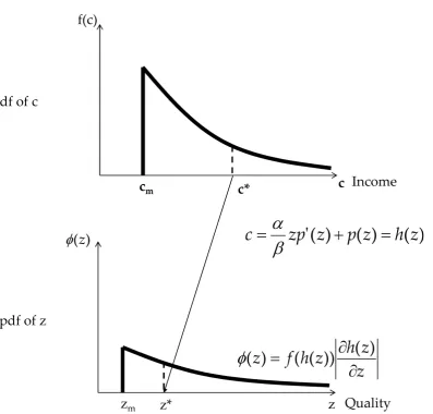
denote the consumer’s income conditional on choosing quality z by h(z). Recalled that f(c) denotes the pdf of income c, and that c = h(z) whence z = h−1(c). From this we can write down the pdf ofz, which we denote as

φ(z), as follows:

φ(z) = f(h(z))

∂h(z) ∂z

(2.1)

where|·|denotes the absolute value and is used to ensure thatφ(z)is always

positive even if∂h(z)/∂z<0.

Figure 2.1: Mapping From Income Distribution to Distribution of Quality Demanded

Substituting forh(z)and f(·)in (2.1) yields

φ(z) = f(α βzp

0₍

z) +p(z))

∂(α_βzp0(z) +p(z)) ∂z

= f(α

βzp

0₍

z) +p(z))

α β(p

0₍

z) +zp00(z)) +p0(z)

= kcckmc(

α βzp

0₍

z) +p(z))−(kc+1)

α β(p

0₍

z) +zp00(z)) +p0(z)

interval:

Qd(z)dz=kcckmc(

α βzp

0₍

z) +p(z))−(kc+1)

α β(p

0₍

z) +zp00(z)) +p0(z)

dz

2.1.2

The Producer’s Problem

On the supply side, there is a unit mass of firms producing vertically dif-ferentiated goods indexed by their product quality z. The distribution of the firms is assumed to be the Pareto distribution characterized by two pa-rameters kz and zm, where zm is the lower bound of z and kz is the shape

parameter.2 The pdf ofzis assumed to take the form:

g(z) = kz z kz m

zkz+1,kz >0,z∈ [zm,∞)

Producers in all countries are assumed to have the same cost function

∆(M,z) = AzMτzγ,τ > 1,γ > 1, where Az is the productivity parameter

and M denotes the number of units of the product with quality z that the firm produces. We assumeτ >1 andγ>1, which ensures that total cost is

a convex function inMandz.

The producers are price takers. Furthermore, it is assumed that the pro-ducers can varyMbut notz. (i.e. a producer’s quality is a given parameter in the short run). Therefore, the producer’s problem is to maximize profit by choosing its output level Mof the quality good:

2_{The reasons for using the Pareto distribution are not only that we can get a closed form}

max

M Mp(z)−∆(M,z)

The first-order conditions imply that

p(z) = ∂∆

∂M =AzτM

τ−1_zγ

Thus, M(z) = ( p(z)

Azτzγ)

1 τ−1

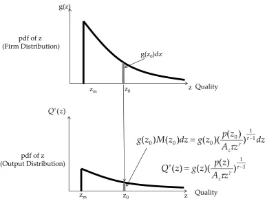
If we denote the firm’s output of the quality good as Qs(z), then the market supply in a small interval dz near qualityz is given by the product of the pdf of firms around z, the quantity supplied by each z firm and the length of the interval:

Qs(z)dz =g(z)M(z)dz

Qs(z)dz =kz z kz m

zkz+1(

p(z)

Azτzγ)

1 τ−1dz

g(z)

z zm

z zm

pdf of z (Firm Distribution)

pdf of z (Output Distribution)

z0

g(z0)dz

dz

z

A

z

p

z

g

dz

z

M

z

g

0

)

(

)

(

)(

(

)

)

(

=

γ

τ

)

)

(

)(

(

)

(

=

γ

τ

z

A

z

p

z

g

z

Q

Figure 2.2: Mapping From Firm Distribution to Distribution of Quality Sup-plied

2.1.3

Market Equilibrium

An equilibrium is defined as a triple {z(c),M(z),p(z)}, where z(c) is the policy functions for consumers, andM(z)for producers, and the price sched-ulep(z)such that:

(1)z(c)solves the consumer’s utility maximization problem taking p(z)

as given.

(2) M(z)solves the producer’s profit maximization problem taking p(z)

as given.

(3) Market clears: demand is equal to supply for z goods, i.e., Qs(z) =

2.1.4

Solving Equilibrium

In equilibrium, we must have the market clearing condition Qs(z)dz =

Qd(z)dz. Therefore,

kz z kz m zkz+1(

p(z)

Azτzγ) 1 τ−1dz

=kcckmc(α_βzp0(z) +p(z))−(kc+1)

α β(p

0_{(z) +zp}00_{(z)) +p}0_(z)

dz

kzzkmz(_A1_zτ) 1

τ−1z−(kz+1)−γτ−11p(z)τ−11

=kcckmc(α_βzp0(z) +p(z))−(kc+1)

α β(p

0_{(z) +zp}00_{(z)) +p}0_(z)

(2.2)

This is a second-order nonlinear non-autonomous differential equation defining p(z),z∈ [zm,∞). We impose a boundary condition:

cm = α

βzmp

0₍

zm) +p(zm)

Herezm is the lowest quality that is viable in the equilibrium, which is

de-termined by the lowest incomecmand the equilibrium price function p(z).

There is no general procedure to obtain the solution of this class of dif-ferential equations, so we adopt the standard method of undetermined co-efficients, to find a particular solution. We postulate the equilibrium price function is of the form p(z) = bzd, withd>0. We then substitute this form of solution into the market clearing condition to solve for the values of the parameterbandd.

The first and second derivatives of the postulated price function form are

p0(z) = bdzd−1,p00(z) = bd(d−1)zd−2 (2.3)

kzzkmz(_Ab_zτ) 1

τ−1z−(kz+1)+(d−γ)(τ−11)

=kcckmc(b(α_βd+1))−(kc+1)(α_βd2+d)bz−d(kc+1)+d−1 (2.4)

Since (2.4) holds for allzand both LHS and RHS are power functions of z, it must be true that the two parameters of the power functions on both sides are equal

kzzkmz(

b Azτ)

1

τ−1 =k_cck_mc(b(α

βd+1))

−(kc+1)₍α

βd

2_{+d)b (2.5)}

−(kz+1) + (d−γ) 1

τ−1 =−d(kc+1) +d−1 (2.6)

From (2.6):

d =

kz+γ

1

τ−1

kc+_τ−1₁

(2.7)

Given Equation (2.7), the expenditure share on zgoods can be obtained by

p(z)

c =

p(z)

α βzp

0_{(z) +p(z)} =

bzd

α βbdz

d_+bzd =

1

α βd+1

(2.8)

From (2.7), (2.8) and the fact thatGini = _2k1

c−1for the Pareto distribution,

we can derive how the Gini coefficient affects the convexity of the price function and hence the expenditure share, which is stated in Proposition 1.

Proposition 1 (Income Distribution and Expenditure Share) Income inequality

has a positive impact on the expenditure share of x goods and a negative impact on

the expenditure share of z goods. Per capita income has no impact on expenditure

shares.

co-efficient implies an increase in d and hence a more convex price function. Since the price ofxis 1 andzhas a non-linear price function, an increase in the convexity of the price function ofzwill make people spend less fraction of their expenditure onzand more onxdue to the high substitutability be-tween the two goods. This mechanism about how income inequality affects expenditure share is crucial in determining how income inequality influ-ences the price level, which will be provided in the next section.

Substituting (2.7) into (2.5) can solve for the other parameter b in the price function:

b = (

kcckmc(α_β

kz+γ(_τ−1₁)

kc+_τ−11

+1)−kckz+γ( 1 τ−1) kc+_τ−11

kzzkmz(_A1_zτ) 1 τ−1

)

1 kc+ 1

τ−1 (2.9)

Therefore, one solution to the differential equation is

p(z) =bzd= (

kcckmc(α_β

kz+γ( 1

τ−1) kc+_τ−11

+1)−kckz+γ( 1 τ−1) kc+_τ−11

kzzkmz(_A1_zτ) 1 τ−1

)

1 kc+ 1

τ−1z kz+γ( 1

τ−1)

kc+ 1

τ−1 ,z∈ [z_m,∞)

wherezm satisfies

cm = α

βzmp

0₍

zm) +p(zm)

After obtaining the equilibrium price function, before aggregating it and analysing how income distribution influences the national price level, we can first investigate how income distribution affects prices at product level, i.e. how the difference in income distribution affects the relative price of a product with a particular qualityz0between two countries.

Suppose the hedonic price functions in country i and country j arepi(z) =

bizdi and pj(z) = bjzdj, wherebi,bj,diand dj are determined as in the

between the two countries is

pi(z0)

pj(z0)

= bi

bj

z(₀di−dj)

If we keep the income distribution of country j constant, and increase the per capita income of country i while keeping its Gini coefficient constant, this will imply an increase in bi and hence an increase in the price ratio for

all values ofz0. If we keep the income distribution of country j constant, and

increase the Gini coefficient of country i while keeping its per capita income coefficient constant, this will imply a decrease in bi and an increase in di.

The increase in di will imply a higher convexity of the price ratio function.

When there are changes in both per capita income and the Gini coefficient, the direction of the change in b will depend on the values of the parameters while the positive relationship between d and the Gini coefficient still hold.

The above results can be formalized as follows:

Proposition 2 If the price ratio of the same good between two countries i and j

pi(z0)

pj(z0) is a function of the quality of that good z0, then the difference in income

in-equality between the two countries determines the power of the price ratio function.

Specifically, if the Gini coefficient of country i is higher (lower) than that of country

j, then the price ratio function is upward (downward) sloping.

We now explore the implications of Proposition 1 and 2 for the B-S rela-tionship, in two alternative settings:

(a) Perfect quality measurement.

(b) A setting where quality is not measured as in Pakes (2003).

goods and the price schedule of the zgoods p(z). Then the price schedule p(z)can be used to construct a price index of the zgoods. Finally, the unit price of the x goods and the price index of thezgoods are aggregated into a national price level. The above procedures of measurement and aggre-gation face, however, a prominent practical issue. The issue is that quality cannot be perfectly controlled for the zgoods. Pakes (2003) shows how to use hedonics to adjust quality biases in the price indexes of quality goods due to the introduction of new goods. The adjustment procedures require a complete dataset on the characteristics of the goods, which is impossible in reality. Without the level of quality being observed, the observed prices of thez goods cannot tell us anything about the price level of thez goods, as their prices depend on both the level of qualityzand the parameters band d in the price function. The measurement issue at the data collecting stage will also contaminate the aggregation procedure. Without knowing the un-derlying price schedule p(z), the common practice of constructing the price index of thezgoods is to use the simple average of the observed prices as its price index. As a result, a higher price index of thezgoods could be either due to higher values of b and d in the price function or simply due to the fact that the prices of higher quality goods have been observed.

Suppose quality can be properly measured, which means that we are able to reveal the underlying price function p(z), then equation (2.9) im-plies that there still exists the B-S relationship. To see this, suppose we keep a country’s Gini index constant and increase its per capita income, this im-plies a constantkcbut a highercm in the Pareto distribution. From (2.7) and

output will increase their prices as the marginal cost is increasing in output. The elasticity of b with respect to cm is equal to _k kc

c+_τ−11

. Given reasonable values of the parameters, the elasticity is quantitatively small.

If quality cannot be adjusted as in Pakes (2003), we have to use the sim-ple average of the observed prices of thezgoods as its price index. Suppose we again keep a country’s Gini index constant and increase its per capita income, now the price index of the z goods not only reflects a higherb as in the previous situation but also reflects the fact that now the country will consume goods with higher qualities than before. This will cause an up-ward bias in the price index of the zgoods and hence in the national price level. Moreover, as income inequality can affect the convexity of the price function and the expenditure share on z goods as shown in Proposition 1 and 2, it will have an impact on the price index of thez goods and the na-tional price level. The details are shown in the next section.

2.1.5

Aggregate Price Level

Given the market equilibrium price schedule p(z), we can calculate the av-erage price level of z goods p, which is the total expenditure on z goods divided by the total number of units.

p=

R∞

zmp(z)Q s_(z)dz

R∞

zmQ s_(z)dz

=

R∞

zmbz d_k

zzkmz(_Ab_zτ) 1

τ−1z−(kz+1)+(d−γ)( 1 τ−1)dz

R∞

zmkzz kz m(_Ab_zτ)

1

τ−1z−(kz+1)+(d−γ)( 1 τ−1)dz

=b

R∞

zmz

−(kz+1)+(d−γ)(_τ−1₁)+d_dz

R∞

zmz

=b

z−(kz+1)+(d−γ)(τ−11)+d+1 −(kz+1)+(d−γ)(_τ−1₁)+d+1 |

∞

zm

z−(kz+1)+(d−γ)(τ−11)+1 −(kz+1)+(d−γ)(_τ−1₁)+1 |

∞

zm

If we assume−(kz+1) + (d−γ)(_τ−1₁) +d+1<0, then

p = −(kz+1) + (d−γ)(

1

τ−1) +1

−(kz+1) + (d−γ)(_τ−1₁) +d+1

bzmd

Sincecm = α_βzmp0(zm) +p(zm)and p(z) =bzd,bzdm =

β

αd+βcm, we have

p= −(kz+1) + (d−γ)(

1

τ−1) +1

−(kz+1) + (d−γ)(_τ−1₁) +d+1 β

αd+βcm (2.10)

Substituting (2.7) into (2.10), we have

p = kc

kc−1

cm β

αkz

+γ(_τ−1₁)

kc+_τ−11

+β

Since the Gini coefficient and the mean of the Pareto income distribution are equal to _2kc1₋₁ and kccm

kc−1, we can express the average price level in terms

of the mean and the Gini coefficient

p=µ β

αkz

+γ(_τ−1₁)

1 Gini+1

2 +τ−11

+β

(2.11)

where µ = _kck₋c₁cm and Gini are the mean and the Gini coefficient of the

income distribution. This equation tells us the effects of per capita income and income inequality on the average price level of z goods, which is sum-marized in Proposition 3.

Proposition 3 (Income Distribution and the Disaggregate Price Level) Per capita

income has a positive impact on the average price level of z goods, whereas income

z goods with respect to per capita income is positive and its semi-elasticity with

respect to income inequality is negative.

Proo f: See Appendix 2.1.

Equation (2.11) also shows that the effect of per capita income on the average price level ofz goods depends on income inequality and the effect of income inequality depends on per capita income.

Proposition 4 The effect of income inequality on the average price level of z goods

(the absolute value of ∂p

∂Gini) is increasing in per capita incomeµ, while the effect of

per capita income on the average price level of z goods (∂p

∂µ) is decreasing in income

inequality.

Proo f: See Appendix 2.2.

To investigate the implications of income distribution for the national price level, we need to construct an aggregate price index.

Although the vertically differentiated goods are produced by local firms, the homogeneous goods are tradable goods with their price level equal-ized across countries. Therefore, the cross-countries price comparison is still meaningful as we can compare the national price level using the price level of the homogeneous goods as an anchor or a numeraire.

Here for simplicity and in order to derive analytical results, we define the aggregate price level as the average price of x goods and z goods weighted by expenditure shares as in the Laspeyres or Paasche index. In Proposition 5, the results regarding how income distribution affects the aggregate price level are shown.

To make the results comparable with the empirical evidence, the results regarding how income distribution affects the log of the aggregate price level are also shown.

(a) Income Distribution and the Paasche Index: If we define the aggregate price

as the Paasche index

PP =

1

1sharex+ p

p₀sharez =1

αd αd+β+

p p₀

β αd+β,

where zero is used in the subscript to denote the variables from the base country,

i.e. the U.S., then per capita income has a positive impact on the aggregate price

level, or the elasticity of the aggregate price level with respect to per capita income

(ePP,µ ≡ ∂PP

∂µ µ

PP) is positive. Moreover, the impact of income inequality on the

aggregate price level and the semi-elasticity of the aggregate price level with respect

to income inequality (ePP,Gini ≡

∂PP

∂Gini

1

PP) depend on the per capita income relative

to the U.S.. They are both positive when per capita income is low enough relative to

the U.S. while they are both negative when per capita income is high.

(b) Income Distribution and the Laspeyres Index: If we define the aggregate

price as the Laspeyres index

PL = 1

1sharex,0+ p

p₀sharez,0 =1

αd0

αd0+β+

p p₀

β αd0+β.

Then per capita income has a positive impact on the aggregate price level, i.e. the

elasticity of the aggregate price level with respect to per capita income (ePL,µ ≡ ∂PL

∂µ µ

PL) is positive, whereas income inequality has a negative impact, or the

semi-elasticity of the aggregate price level with respect to income inequality (ePL,Gini ≡

∂PL

∂Gini

1

PL) is negative.

(c) No matter whether the aggregate price level is defined as the Laspeyres index

or the Paasche index, the effect of per capita income on the aggregate price level

(∂PP

∂µ and ∂PL

∂µ) is decreasing in income inequality and the effect of income inequality

( ∂PP

∂Giniand ∂PL

∂Gini) is decreasing in per capita incomeµ. Moreover, the elasticity of the

aggregate price level with respect to per capita income ePP,µ and ePL,µis decreasing

respect to income inequality ePP,Giniand ePL,Giniis decreasing in per capita income

µ.

Proo f: See Appendix 2.3.

In practice, the way to construct the multilateral price index as in the International Comparison Program (ICP) is different. However, as shown in Deaton and Heston (2010), it can be approximated very well by the bilateral Fisher index, i.e., a geometric mean of the Laspeyres and the Paasche index. Therefore, the results in Proposition 5 can be used to show how income distribution affects the bilateral Fisher index or the national price level.

No matter whether the aggregate index is defined as the Laspeyres index or the Paasche index, the elasticity of the national price level with respect to per capita income is always positive and it is decreasing in income in-equality. Since the elasticity of the Laspeyres index with respect to income inequality is negative and the elasticity of the Paasche index with respect to income inequality is decreasing in per capita income, with a low enough per capita income, the elasticity of the bilateral Fisher index could be posi-tive while it is negaposi-tive with a high per capita income. This is confirmed in Figure 2.3, where the derivatives of the bilateral Fisher index with respect to income inequality ∂PF

∂Gini for different combinations of per capita income and

income inequality are plotted. For a lower level of per capita income ∂PF

∂Gini is

positive, while it is negative when per capita income is high.

expen-−0.4

−0.35

−0.3

−0.3

−0.25

−0.25

−0.2

−0.2

−0.2

−0.15

−0.15

−0.15

−0.1

−0.1

−0.1

−0.05 −0.05

−0.05

0

0

0

0.0 5

Per Capita Income

Gini

0.5 1 1.5 2 2.5 3 3.5 4 4.5 5

x 104

0.2 0.25 0.3 0.35 0.4 0.45 0.5

Figure 2.3: The Contour of the Effect of Income Inequality on the Bilateral Fisher Index ( ∂PF

∂Gini) for Different Combinations of Per Capita Income and

Income Inequality.

Notes: The base country income distribution is calibrated using U.S. data in 2003.

expenditure share on z goods will reduce the aggregate price level. Since the product of the expenditure share and the average price of z enters the aggregate price level, a higher per capita income, which increases the aver-age price ofz, will strengthen the effect of income inequality, while a lower income inequality, which increases the expenditure share of z, strengthens the effect of per capita income. Hence the effect of per capita income must be decreasing in income inequality and the effect of income inequality must be decreasing in per capita income.

Next, we ask: what is the key feature of the present model that leads to Proposition 5. To address this question, we develop in Appendix 2.4 an alternative model based on the classic model of vertical product differenti-ation.

As quality is not controlled for in the price index of quality products, the price index of quality products is measured as the average expenditure on quality products. Keeping per capita income constant, the price index of quality products will only depend on its expenditure share. Therefore, whether income inequality can affect the price index of quality products crucially depends on whether income inequality can affect the expenditure shares.

the expenditure share. Therefore, the price index of quality products will be affected by income inequality. Since the national price level is a weighted average of the price levels of the quality products and commodity goods, the national price level will also be affected by income inequality.

2.2

Empirical Tests I: Income Distribution and the Aggregate Price

Level

This model predicts the B-S relationship, but it also predicts a new rela-tionship between income inequality and the national price level, which is summarized in Proposition 5 above. The new relationship is as follows:

Controlling for per capita income, income inequality is correlated with the national price level: within countries with lower per capita income, in-come inequality is positively correlated with the national price level, while within countries with higher per capita income, the correlation is negative.

In this section, we investigate this prediction directly. In the next section, we investigate some additional predictions of the model that follow from Proposition 1 and 3.

Figure 2.4: Price Level versus GDP per capita in 2003 (U.S.=1)

Notes: Source: The Penn World Table 6.2

First, the figure in Rogoff (1996) is reproduced in Figure 2.4 using 2003 data.3 The data on prices and income are from Penn World Table PWT 6.2. The data on the Gini coefficients are taken from the World Bank: World Development Indicators 2007. Figure 2.4 shows that the problem with the Balassa-Samuelson hypothesis still persists; it performs well for the whole sample, but does not perform well either within poor countries or within rich countries.

3_{Data from 2003 is used because cross-sectional Gini coefficients from World}

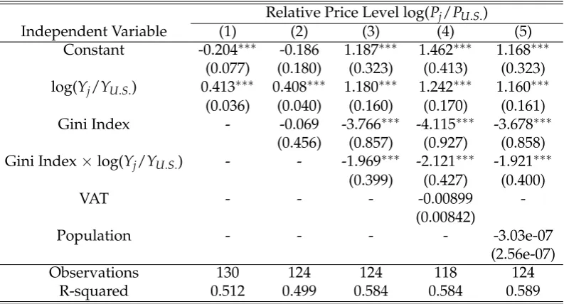
Table 2.1: The Effects of the Gini Coefficient in 2003

Relative Price Level log(Pj/PU.S.)

Independent Variable (1) (2) (3) (4) (5)

Constant -0.204∗∗∗ -0.186 1.187∗∗∗ 1.462∗∗∗ 1.168∗∗∗

(0.077) (0.180) (0.323) (0.413) (0.323)

log(Yj/YU.S.) 0.413∗∗∗ 0.408∗∗∗ 1.180∗∗∗ 1.242∗∗∗ 1.160∗∗∗

(0.036) (0.040) (0.160) (0.170) (0.161)

Gini Index - -0.069 -3.766∗∗∗ -4.115∗∗∗ -3.678∗∗∗

(0.456) (0.857) (0.927) (0.858)

Gini Index×log(Yj/YU.S.) - - -1.969∗∗∗ -2.121∗∗∗ -1.921∗∗∗

(0.399) (0.427) (0.400)

VAT - - - -0.00899

-(0.00842)

Population - - - - -3.03e-07

(2.56e-07)

Observations 130 124 124 118 124

R-squared 0.512 0.499 0.584 0.584 0.589

Note: Data on price and income are taken from the Penn World Tables 6.2. Data on the Gini Index are taken from World Bank: World Development Indicators 2007. VAT data is from International VAT and IPT Service. Population data is from WRDS.

∗∗∗_,∗∗ _and∗ _{indicate statistically significant different from zero at 1%, 5% and 10%}

level respectively.

which has significant explanatory power, the estimated coefficient of the Gini index will be the sum of the estimated coefficient of the Gini index in Regression (3) and the product of the estimated coefficient of the interaction term in Regression (3) and the relative income. Since in the sample, most of the relative incomes in logarithm are negative, when they are multiplied with the negative coefficient of the interaction terms, they reduce the mag-nitude of the negative coefficient of the Gini index and make it insignificant in Regression (2). Therefore, the results show that per capita income has a positive impact on the aggregate price level, i.e. the Penn effect, while in-come inequality also has a significant impact on the aggregate price level and the impact is decreasing in per capita income. These are consistent with the model predictions in Proposition 5 that per capita income has a posi-tive impact on the national price level and the impact of income inequality on the national price level is decreasing in per capita income. Regressions

(4) and (5) control for VAT and population, with the latter being a proxy for market size. The estimation results show that the inclusion of these two control variables does not change the estimation result in (3). Moreover, both control variables are not significant at the 10% level.

Table 2.2: Different Behaviors of Income Distributions in Different Samples in 2003

Relative Price Level log(Pj/PU.S.)

Threshold=0.33 ofYU.S Threshold=0.60 ofYU.S

Poor Countries Rich Countries Poor Countries Rich Countries

Independent Variable (1) (2) (3) (4) (5) (6) (7) (8)

Constant -0.899∗∗∗ -1.376∗∗∗ 0.256∗∗∗ 0.999∗∗∗ -0.713∗∗∗ -0.978∗∗∗ 0.154∗∗ 1.066∗∗∗

(0.124) (0.223) (0.085) (0.224) (0.107) (0.204) (0.074) (0.168)

log(Yj/YU.S.) 0.157∗∗∗ 0.159∗∗∗ 0.915∗∗∗ 0.910∗∗∗ 0.223∗∗∗ 0.234∗∗∗ 0.361 0.378∗

(0.049) (0.048) (0.181) (0.145) (0.044) (0.046) (0.230) (0.205)

Gini Index - 1.113∗∗ - -2.125∗∗∗ - 0.684 - -2.721∗∗∗

(0.440) (0.632) (0.441) (0.477)

Observations 96 95 34 29 105 102 25 22

R-squared 0.097 0.154 0.444 0.642 0.196 0.211 0.097 0.660

Note: Data on price and income are taken from the Penn World Tables 6.2. Data on the Gini Index are taken

from World Bank: World Development Indicators 2007. ∗∗∗,∗∗and∗indicate statistically significant different

from zero at 1%, 5% and 10% level respectively.

to a one percentage point increase in per capita income, whereas the price level decreases by about 2.72 percent with the 95% confidence interval being

[1.723, 3.719]in response to a one hundred basis points increase in the Gini coefficient. Moreover, as the Gini coefficients are usually measured with large errors, the magnitude of the estimate is probably biased downwards.

As have been shown in the model, the positive relationship between per capita income and the national price level in Table 2.1 is due to the fact that quality is not controlled for. For example, in Bils and Klenow (2001), they use the U.S. data to show that quality growth of 66 durable goods causes an over-estimation of inflation by 2.2%. If quality cannot be controlled for, then it will show up in the price index. Moreover, due to the fact that income elasticity of quality for many consumption goods are non-negligible and tend to be higher for nontraded goods, which are priced in a non-linear way, income distribution will matter for people’s choice of quality and will affect the national price level through the price of nontraded goods. This is why income inequality also affects the measured national price level.

2.3

Empirical Tests II: Income Distribution, Disaggregate Price

lev-els and Expenditure Shares

In this section, we examine the further predictions of the model that follow from Proposition 1 and 3. For convenience, we repeat the statements of these propositions as follows:

Proposition 1 (Income Distribution and Expenditure Share) Income inequality

has a positive impact on the expenditure share of x goods and a negative impact on

the expenditure share of z goods. Per capita income has no impact on expenditure

shares.

income has a positive impact on the average price level of z goods, whereas income

inequality has a negative impact. Therefore, the elasticity of the average price of

z goods with respect to per capita income is positive and its semi-elasticity with

respect to income inequality is negative.

These propositions can be tested using a 2-step procedure, as follows: Step 1: Using consumption expenditure data, we can identify which good in the consumption bundle is more like the x goods and which good is more like thezgoods.

Step 2: To test if the empirical effects of income distribution on the price level and expenditure share of thexand zgoods are the same as predicted in Proposition 1 and 3.

Since the aggregate price level is an average price level of consumption weighted by expenditure shares, we have to understand the aggregation methods used in practice in order to show that both the assumptions in the model and the model mechanism are consistent with the data. In the con-struction of both national price indices such as the CPI and multilateral price indices in the Penn World Table, the first step is to construct the sub-indices for different components of consumer expenditure. Then, expenditure data from each country’s national account is used to construct the weights for dif-ferent components and all the sub-indices are aggregated into an aggregate price index using these weights. However, some aspects of this aggregation method can have important consequences.

observation combined with the aggregation method can have two conse-quences. Firstly, due to the lack of data on the characteristics of goods, the aggregation method is not able to control quality, hence the higher quality of z goods will be translated into a higher price. Secondly, as has already been shown in the model, income inequality affects the price function and the expenditure share ofzgoods, and hence the aggregate price level.

Guided by the dichotomy of xand zgoods, to understand how income distribution influences the aggregate price level, Section 2.3.2 investigates how disaggregate prices and expenditure shares change with income dis-tribution, which can be used to show that the mechanism of the model is consistent with the data.

2.3.1

Identification of x goods and z goods

In the traditional literature, prices usually do not play a role and consump-tion (physical quantity) is equivalent to consumpconsump-tion expenditure given that the price function is linear and unit price is constant. Hence the income elasticity for one good is the income elasticity of consumption (or consump-tion expenditure) for that good.

However, in this chapter, because a type zgood is priced in a non-linear way, the equivalence between consumption and consumption expenditure is broken.

of quality (unit price) as follows:

eexpenditure =

dlog(consumption expenditure)

dlog(income)

= dlog(quantity×unit price)

dlog(income)

= d[log(quantity) +log(unit price)]

dlog(income)

= dlog(quantity)

dlog(income) +

dlog(unit price)

dlog(income) = equantity+equality

is important to incorporate the dichotomy ofx goods andz goods into the model due to its significant expenditure share.4

Table 2.3: Expenditure Shares of Food, Housing, Apparel, Transportation and Restaurants and Hotels

Country Share of Share of Share of z goods

the Five Categories z goods within the Five Categories

Max 0.751 0.508 0.805

Min 0.466 0.314 0.632

Average 0.606 0.426 0.703

Standard Deviation 0.051 0.043 0.042

Food

As has been documented in the literature, calorie intake does not vary with permanent income across households. Specifically, Aguiar and Hurst (2005) find that employed household heads with a higher income consume simi-lar amounts of calories as employed household heads with a lower income. However, conditional on log calories, they find that the income elasticities of vitamin A and vitamin C are over 0.30 and the income elasticities of vi-tamin E and calcium are 0.17 and 0.08, respectively. In addition, the income elasticity of cholesterol is negative.

The results suggest that the income elasticity of quantity for food is very close to zero. Households with higher income do not consume a larger quantity of food than households with lower income. Instead, they con-sume higher quality foods, such as those rich in vitamin and calcium. On the other hand, low income households consume cheaper calories by having a higher composition of fat and cholesterol in their diets.

4_{Since food at restaurant is a substitute of food at home and staying at a hotel is a}

Housing

As has been defined previously, the number of houses counts as quantity whereas other characteristics of a house, such as square meters, all count as quality. Micro-evidence has shown that the price function of housing is nonlinear. For example, Anderson (1985) estimates the hedonic price func-tion of housing, i.e. regressing the housing price on characteristics of the house which include structural characteristics of the house, improvements to the house, physical characteristics of the lot, neighbourhood character-istics, etc. He shows that the price function is convex. Even if we define housing by square meters, the price function is still estimated as a convex function. For example, Coulson (1992) estimates a nonparametric response of housing price to floorspace size. The marginal price is estimated to be in-creasing, which implies a convex price function. Mason and Quigley (1996) estimate the hedonic price indices for downtown Los Angeles and they find the price function is convex in size (1000 sq ft). Also, Bao and Wan (2004) find that the sale price per square foot is increasing in gross area controlling for other characteristics using Hong Kong data.

We use data from the SCF (Survey of Consumer Finances) to compute the number of residences, total value of residences and value per residence by percentile of income. Figure 2.5 plots the results for the year 2004.

(a) Number of Residences

(b) Total Value of Residences (thousands of dollars)

(c) Value Per Residence (thousands of dollars)

Clothes

The detailed expenditure data on clothes are extracted from the raw data files of the Consumer Expenditure Survey (CEX), which includes both the expenditure on and quantity of clothes. The total expenditure on a certain type of clothes is divided by the number of clothes to get the unit price. Figure 2.6 plots the total expenditure and the unit price for different types of clothes across the nine income classes in the CEX. The white bars denote the total expenditure and the black bars denote the unit price. It can be seen that for all types of clothes, unit prices are almost the same for all income classes, which suggests a very low income elasticity of quality.

Vehicle

Data on the quantity and expenditure of vehicles is also available from the CEX. As has been done for housing, Figure 2.7 plots the number of vehicles, total value of vehicle purchases and unit value per vehicle across income classes. It shows that neither income elasticity of quantity nor income elas-ticity of quality is zero. As we move from lower income groups to higher income groups, both quantity and quality increase significantly.

(a) Coats (b) Sweaters

(c) Pants (d) Shirts

(e) Undergarments (f) Hosiery

(g) Footwear

Figure 2.6: Total Expenditure and Unit Price for Different Types of Clothes in Dollars (CEX 2003).

(a) Number of Vehicles

(b) Total Value of Vehicles (dollars)

(c) Value Per Vehicle (dollars)

In summary, the evidence presented shows that the income elasticities of quantity of food and housing are close to zero, the income elasticity of qual-ity of clothes is close to zero and both are nonzero for vehicles. Some may argue that the observed two elasticities are equilibrium outcomes, which are endogenous. Hence, the observed patterns cannot be taken as primitives in the model. However, the observed elasticities, especially the zero income elasticity of quantity of food and housing, are not due to equilibrium out-comes, but instead, are due to the nature of the goods. For example, the daily calorie intake has to be within a certain range regardless of income and for convenience, a household usually has one primary residence. Finally, given the fact that the tradability of food and housing is generally lower than that of clothes and vehicles, it is reasonable to assume thatxgoods are tradable with the price normalized to 1 andzgoods are non-tradable with a non-linear price function.

2.3.2

The Impact of Income Distribution on the Price Levels of

In-dividual Product Groups and Expenditure Shares

Since the national price level is an average price level of disaggregate price levels weighted by expenditure shares. By examining how disaggregate price levels and expenditure shares vary with income distribution, we can trace out the main drivers of the positive relationship between per capita income and the national price level, and, more importantly, the relationship between income inequality and the national price level.

In this subsection, we investigate empirically how income distribution affects disaggregate price levels and expenditure shares. This leads to direct tests of the model’s predictions in Proposition 1 and 3.

However, in practice, few goods are pure x or pure z. Nevertheless, we can quantify the degree to which a good belongs toxorzbased on the fea-tures of these two types of goods. The prices of thexgoods are assumed to be equalized across countries and the prices of the z goods are locally de-termined and related to local per capita income. We can therefore use the elasticity of a product’s price with respect to per capita income, which is designated here as the quality index of the product, to measure whether the product is more like axgood or azgood.

As the most disaggregate level of the PPP data from the ICP is the basic heading level, we first compute the quality index for each basic heading by running cross-country regressions, by regressing the log of the price levels of one product on the log of countries’ per capita income.

Then we regress the disaggregate price level on per capita income, the Gin coefficient and the product of per capita income and the Gini coefficient for each basic heading using the underlying PPP data from the ICP5 and show how the estimation results vary from the basic headings with high quality index to the basic headings with low quality index.

log(Pricei) = β0+β1log(Per Capita Income) +β2Gini

+β3log(Per Capita Income)·Gini+ei

To do so, we plot the estimated coefficient from the above regression against the quality index to see how the latter affects the coefficient of per capita income, the Gini coefficient and the interaction term. Panel (a), (b)

5_{The dataset used here is from the ICP benchmark 2005, which provides disaggregate}

and (c) in Figure 2.8 plot these estimated coefficients, i.e. ˆβ1, ˆβ2 and ˆβ3,

against the quality index.

(a) ˆβ1vs Quality index (b) ˆβ2vs Quality index

(c) ˆβ3vs Quality index (d)Corr(Expenditure Share,Gini) vs Quality

Index

Figure 2.8: How the Quality Index Affects the Impact of Income Distribu-tion on the Price Level of Individual Product Groups and Expenditure Share (Source: ICP 2005)

Notes: The size of markers in the above scatter plots is proportional to the average

An Examination of Product Level Data

3.1

Introduction

Chapter 2 is devoted to exploring the Balassa-Samuelson relationship at the aggregate level. To further understand the sources of the aggregate relation-ship at the disaggregate level, in this chapter, we take a purely statistical approach in asking the question: what is the best statistical description of the relationship between wealth and the price levels of individual products. The motivation of doing so is that the huge variations in the aggregate B-S relationship across countries with different levels of income imply that using the B-S hypothesis as the single general theory to explain national price levels is far from satisfactory. The driving forces of the huge variations are crucial to understand the aggregate price level. For example, Rogoff (1996) has shown that there is empirical support for it when comparisons are made between the set of poor countries and the set of rich countries. However, its explanatory powers are far less impressive within either the poor countries group or the rich countries group. As shown in Chapter 2, regressing the national price level on per capita GDP generates an R2 of 0.51 in the whole sample. When the whole sample is split according to per capita income with 60 percent of the US GDP per capita as the threshold, the R2s within the poor countries and the rich countries become 0.20 and 0.10 respectively. In addition to R2, the two countries groups also differ in the elasticity of the national price level with respect to per capita income. Within the poor countries, the elasticity of the national price level with respect to

per capita income is around 0.22, which is far lower than the elasticity of 0.36 within the rich countries. The above two results are robust to the choice of threshold. For example, using one third of the US GDP per capita as the threshold can only affect the results quantitatively but not qualitatively.

Since the national price level is an average of disaggregate price levels weighted by expenditure shares, we can use the underlying disaggregate price levels and expenditure shares to dig out the sources of the variations in the B-S relationship. Our goal in this chapter is to find the cleanest statistical description of the relationship between wealth and the price levels of indi-vidual products. However, testing the Balassa-Samuelson hypothesis using disaggregate price levels is not new in the literature. For example, Heston et al. (1994) use disaggregate price levels to test an intermediate prediction of the hypothesis: the price ratio of tradable to nontradable is decreasing in income. Similar tests can be found in Kravis and Lipsey (1988). These tests did provide empirical support for the hypothesis, but they did not address the variations of the B-S effects across countries and products.

(a) (b)

Figure 3.1: Two Archetypes of Price-Wealth Relationships

We illustrate the two types of relationship in Figure 3.1.

The details about how to quantify the B-S relationship at product level and their theoretical implications will be provided in the next section.

3.2

Empirical Evidence: Characterizing the B-S Relationship at

Prod-uct Level

To get an idea of how the B-S effect varies across products and countries, we first plot the scatter diagram of the price level against GDP per capita (in logarithm) relative to the US for each basic heading in Figure 3.2. On inspection, we can identify a clear and striking empirical pattern: for some products, the B-S relationship is weak and disperse. For example, in the case of

(1) (2) (3) (4)

(5) (6) (7) (8)

(9) (10) (11) (12)

(13) (14) (15) (16)

(17) (18) (19) (20)

(21) (22) (23) (24)

(25) (26) (27) (28)

(29) (30) (31) (32)

(33) (34) (35) (36)

(37) (38) (39) (40)

(41) (42) (43) (44)

(45) (46) (47) (48)

(49) (50) (51) (52)

(53) (54) (55) (56)

(57) (58) (59) (60)

(61) (62) (63) (64)

(65) (66) (67) (68)

(69) (70) (71) (72)