2017 International Conference on Computer Science and Application Engineering (CSAE 2017) ISBN: 978-1-60595-505-6
A Graph Based Method to Mine Frequent Dense Resources across
Multiple Discrete-Value Function-Resource Effectiveness Matrix
Miao Wang1, Talent Paul Mavingire2, Xiangzhen Zan3, Wenbin Liu2 and Liangzhong Shen3*
1
Science and Technology on Avionics Integration Laboratory, Shanghai, China;#2, China National Aeronautical Radio Electronics Research Institute, Shanghai, China
2
Department of Physics and Electronic Information Engineering, Wenzhou University, Wenzhou city, Zhejiang province, China
3
Wenzhou Business College, Wenzhou city, Zhejiang province, China
ABSTRACT
A function plays a pivotal role when it comes to the improvement of system task information. It is the basis for a guarantee of effectiveness and performance of the system. However, this implies that for the function health to be fully effective its resources need also to be up to par. An antagonistic relationship between the function resource and the function health, wherein the resources are of low standard only brings about downgrade in performance and effectiveness of the function. In this paper, we aim to showcase a study on the relation of functions and resources effectiveness from the data of functions' resource effectiveness matrix and how it can excavate the health relation between resources and functions. In previous studies, most methods focused on designing complex algorithms to extract dense connected resources from one function's resource effectiveness matrix. We propose our own method for the mining of frequent dense resources across multiple discrete-value function-resource effectiveness matrix. It has proven to be better as the experimental results show our algorithm can extract frequent dense resource sets that satisfy the specified conditions in a more efficient way.
INTRODUCTION
Over the years, the avionics system’s functional requirements have improved immensely. Such an improvement has led also to enhancement in performance and complexity of the system including the system’s resource requirements. However, the system’s reliability and safety have had a fallout as they are significantly reduced. The assembly of the avionics system becomes more intricate than ever. Thus, the resources’ competence directly influences the effectiveness of the avionics system as damage to them might cause some inefficiencies to the system. Contemporary research has demonstrated that by studying the level of efficiency of resources we obtain the basis for building presage and health management systems [1]. Efficiency level of resources impacts the function level of the system. Studying the call relation of functions and resources effectiveness from the data of functions' resource effectiveness matrix can excavate the health relation between resources and functions.
[2,3]. The second one gives attention on how to mine biclusters with maximal variant usage rate and maximal low usage rate in function-resource matrix [4,5,6,7,8,9,10]. Fewer studies, however, have paid attention on how to mine differential resource patterns from multiple functions’ effectiveness matrixes expeditiously with efficiency given the statistic of different functions performance being based on the different requirements of resource effectiveness. Our study can aid in finding potential hazards when tasked to perform multiple functions simultaneously. A method we propose, that is, to mine frequent dense resources patterns across multiple discrete-value function-resource effectiveness matrix. This will enable us to tackle the above problems.
The paper is organized as follows. Section II introduces the problem formulation and some definitions needed. Section III contains a proposed algorithm to mine frequent dense resources across multiple discrete-value function-resource effectiveness matrix. Going on to section IV, we give the experimental results to demonstrate the validity of the algorithm. Finally, we give the conclusion in section V.
PROBLEM DESCRIPTION
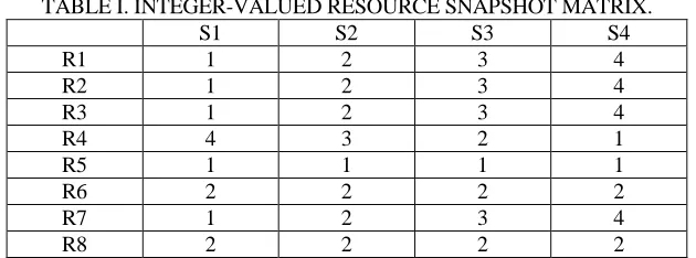
[image:2.612.140.455.377.494.2]A great amount of state monitoring and data processing modules are used in the aircraft for us to effectively analyze the aircraft safety. The resource effectiveness matrix defined as a two-dimensional real matrix D R S is shown in TABLE I.
TABLE I. INTEGER-VALUED RESOURCE SNAPSHOT MATRIX.
S1 S2 S3 S4
R1 1 2 3 4
R2 1 2 3 4
R3 1 2 3 4
R4 4 3 2 1
R5 1 1 1 1
R6 2 2 2 2
R7 1 2 3 4
R8 2 2 2 2
Depicted in the above table, row section R represents the resource name; column
section S references the different sampling sites. ElementDij of matrix D is an integer number which indicates the effective value of resource i under sampling j. To facilitate effective mining, the original valid values in the resource effectiveness matrix can be discretized into 1, 2…. N. Amongst the values, the lowest effectiveness of resources is represented by 1, and N takes on the highest effectiveness of resources. In TABLE I, the value of N is 4.
The function's resource effective matrix can therefore be modeled as a simple unweighted and undirected graph, where each resource is represented by one node and two resources are connected with an edge if their sampling values show the same specified trend (See definition 2).
Definition 1 Assuming the values of resource R1 in two consecutive samples S1 and S2are expressed as V1 and V2, the trend of resource R1in S1 and S2 can be defined.
2. if ,V2 V1 resource R1 represents downtrend between S1 and S2;
3. if V2 V1, resource R1 represents invariance between S1 and S2.
Definition 2 Assuming the values of resource R1 in all the sampling values, the trend of resource R1 can be defined as follows:
1. any two adjacent sampling values are satisfied with the requirements of definition1.1, the trend of resource effectiveness is uptrend;
2. any two adjacent sampling values are satisfied with the requirements of definition1.2, the trend of resource effectiveness is downtrend;
3. any two adjacent sampling values are satisfied with the requirements of definition1.3, the trend of resource effectiveness is invariance;
A densely connected subgraph in such graph may thus correspond to a tight connected resource set with the same trend of effectiveness when the function is performed. Therefore, the problem of mining differential resource patterns from multiple function's effectiveness matrixes can be formulated as:
Given n graphs with m common nodes, search all frequent dense vertexes set
which are densely connected in at least in k graphs (0 k n) . In the following, we present some definitions needed to illustrate our method.
Definition 3 (Graph Set). A graph set D{Gi( ,V Ei)}, 1 i m,Ei V V, where
the graphs in this set share a common vertex set V .
Definition 4 (Graph Density). Consider a graph G V E( , ), its density is defined as
2E /(V V( 1))
, where E and V represent the number of vertices and edges respectively.
Obviously, the density of a graph ranges from 0 to 1. In practice, G is called a dense graph only if ( )G .
In order to mine dense vertex sets, we use the following terms to analyze whether one edge is in the dense connected environment.
Definition 5 (Edge Clustering Coefficient). Given a graph G V E( , ) , the edge clustering coefficient of uvE (u v, V) is defined as [11]
(3) , max( , )
u v uv u v z EC d d (1)
where du and dv represent the degree of vertices u and v respectively,
(3) ,
u v
z
is number of triangles pass through uv.The edge clustering coefficient counts the number of triangles containing a given edge. Although the number of triangles can reflect the density of a subgraph, it does not work well for networks with few short circuits or even no circuits.
Definition 6 (Edge Density Coefficient [12]). Given a graph G( , )V E , the edge density coefficient of uvE (u v, V) is defined as
( 1)( 1) ( ) ( 2) / 2
u v
uv uv
u v
d d
ED g
d d
(2)
where du and dv represent the degree of vertices u and v respectively, guv is the
subgraph induced by edge uv.
dense subgraph with high probability; otherwise, if it is very small, then the edge may bridge between dense subgraphs with high probability.
Definition 7 (Frequent Dense Vertex Set). Given a graph set D{Gi( ,V Ei)}, a set
of vertices V V is a frequent dense vertex set if the density of its induced subgraphs
( ( ))g Vi
is larger than or equal to at least in k graphs.
Definition 8 (Summary Graph). Given a graph set D{Gi( ,V Ei)}, its summary
graph is a graph S V E( , )ˆ where the average edge density coefficient of each edge eEˆ
is larger than a user-defined threshold.
METHODS
The arduous task of mining frequent dense resource sets arises from the fact that the connected dense resource set are concealed among a vast expanse of superfluous edges. The extraneous edges can be defined as those having no contribution to the formation of frequent dense resource sets, and can be divided into five categories: 1) an edge is sparsely connected with other edges; 2) an edge is densely connected only in a few graphs; 3) an edge bridges two densely connected subgraphs in the summary graph; 4) an edge is not present in summary graph; 5) some dense connected edges appear in a
subset of graphs SUB D( ), but their connections in each graph of D SUB D ( ) have no contribution.
Our algorithm can be broken down to four processes :(1) Construct network according to each function's resource effective matrix; (2) Coarse filtering; (3) Clustering subsets of graphs;(4) Refined filtering on those subsets.
We use the Coarse filtering algorithm to single out those edges from 1) to 4). The pseudocode of the Coarse filtering algorithm is as below.
Algorithm 1: Coarse filtering algorithm
Input: Graph set D {G i (V, E )}i (1 i m), Minimal frequent support k, Minimal
Density threshold , User defined parameter f p q, , ;
Output: Summary graph S(V,E)ˆ and the resulted graph dataset D{Gi(V, E )}i ; 1 begin
2 for each graph Gi, filter out edges with EDe/f ;
3 construct summary graph Swith edges satisfying e i
ED pk
(1 i m);4 in summary graph S, filter out edges with ECeq;
5 by only keeping edges satisfying ˆE ' Ei
e e , return S to Gi; 6 repeat 2 to 5 until the summary graph Sdoes not change any more.
7 end
The pseudocode in line 2 of the algorithm singles out those sparsely connected
edges in each individual graphGi. It cancels out those edges whose EDe /f (f 1) to
circumvent eliminating pertinent edges. Line 3 of the pseudocode of the algorithm constructs a summary graph S . The pseudocode in line 4 of the algorithm prunes those
edges bridging two dense subgraphs in summary graph S; Pseudocode in line 5 of the algorithm returns to each graph Gi by reserving those edges that remained in the
Algorithm1 eradicates an excessive amount of extraneous edges whereas algorithm2 is designed to cluster the edges in the summary to obtain the potential subsets of D. The algorithm 2 comprises chiefly of two processes: one of the processes being projecting all vectors to these seed vectors and the other one being the selection of a seed vector with the largest weight to cluster. The pseudocode of algorithm 2 is as below.
Algorithm 2: Finding potential subsets of D
Input: Summary graph S(V, E)ˆ , Minimal frequent support threshold , Graph number
m, Minimal Hamming distance threshold ;
Output: Cluster center set C;
begin
1: assign each edge support vector of eˆEa weight w(ve) 1 , and puts those with Hamming weight m1orm to set A and others to set B;
2: for each edge veBdo
find the subset veSUB(A)A with the maximal score s(v , v )e e , and update their
weight by w(v )e' w(v ) 1/ SUB(A)e' ;
remove ve from B; end for
3: for all edge vectorveA
move those appeared in m from A to B;
end for
4: for each edge veBdo
find the subset veSUB(A)A satisfying s(v , v ) 1e e , update their
weight by
' '
(v )e (v )e (v ) / SUB(A)e
w w w );
remove ve from B; end for
5: A A B;
6: sort vectors vA in decreasing order according to their weight w(v); 7: do
setT=NULL
move the first vector fromA to T;
for each vAdo
if t T
(v, t) / T
h
, then move v from Ato T; decide a cluster center c based on vectors in T and ( )
t Tw c w(t);
add c to set C;
loop while (A!=NULL);
end
sets they may contain. Having a center’s weight being too small will allow us to discard it.
We proceed to refined filtering on those subsets after applying algorithm1 and algorithm 2 to graph sets. This would be our final procedure. A three steps process is
observed : 1) Build a graph set SUB D( ) based on each cluster center cC, and invoke FILTER to perform a refined filtering of irrelevant edges on SUB D( ); 2) Detect dense subgraphs in the resulted summary graphs and output their vertex sets; 3) Merge identical vertex sets and separate some large vertex sets.
RESULTS
We shall make a contrast of the results yielded by the above algorithm and known results in this unit. The hardware environment of the experiment is Intel(R) Core(TM) i5-5200U CPU@ 2.20GHz 2.20GHz and 8G memory; the software environment is Windows 7 Ultimate operating system (64bit);the algorithm programming and operating environment is Visual C++6.0.
Experimental data was taken to be the simulated data. Having this beforehand, we produced 20 functions' resource effective matrix, each function having the same 200 resources. The sampling value of each resource is between 0 and 10 at random, each resource having been sampled 15 times. The original effective value in resource effectiveness matrix is discretized into 1, 2, 3, ...,10 values, that is, the sampling value of
each resource can be discretized into . The rule used in constructing the network is: two resources having one edge should also have the same uptrend. For us to verify the correctness of the algorithm, we use the dividing block idea to create the frequent and dense resource patterns: for resource1 to resource 28, and resource 135 to resource 178, any two resources in function 1, function 3, function 5, function 9, function 11, function 15 and function 19 show an upward trend; for resource30 to resource 58, and resource 109 to resource 138, any two resources in function 2, function 4, function 6, function 7, function 8, function 10 and function 18 show an upward trend; any two resources of the others present an uptrend at the probability pout0.8, 0.7, 0.6 , respectively. Therefore, we get 20 networks at pout0.8, 0.7, 0.6, respectively. Repeat the process above 2 times, then we get another two graph sets, each graph set having 20 networks at pout0.8, 0.7, 0.6.
As we move on to applying the above algorithm, we obtain frequent dense resource sets from each graph set, where the frequent threshold is 0.3, and the density threshold is 0.8,0.6,0.7 respectively.
Rand Index [13] is a measure of the similarity between two data clustering methods. From a mathematical standpoint, Rand Index is related to the accuracy, but is applicable even when class labels are not used. Therefore, we apply the Rand Index to evaluate the ultimate results. The Rand Index is defined as:
a d R
a b c d
(3)
where a is the number of vertex pairs that belong to the same cluster for both partition I and II; b is the number of vertex pairs that belong to the same cluster in
belong to two clusters for partition I, but belong to the same cluster for partition II; d is
the number of vertex pairs that belong to two clusters for both partition I and II. In this paper, partition I refers to the known frequent dense resource sets, while partition II refers to the frequent dense resource sets obtained by our algorithm.
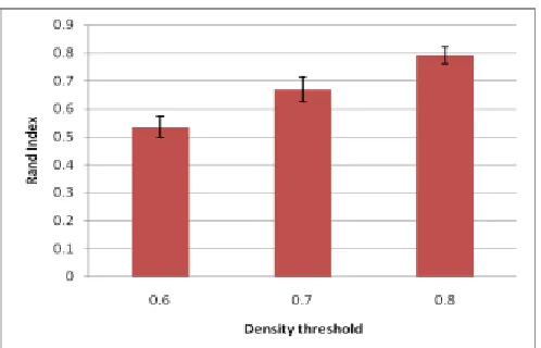
[image:7.612.176.420.166.337.2]Notably, the larger the Rand Index, the more likely that the final partition is consistent with the prescribed community structures. The comparison result is shown in Figure 1, Figure 2, Figure 3.
Figure 1. The average Rand index distribution of the algorithm based on three datasets at density threshold=0.6, 0.7, 0.8, respectively, in the environment at pout=0.6.
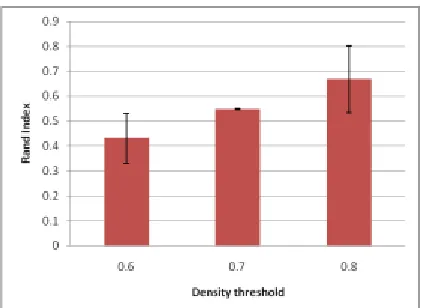
[image:7.612.174.423.377.537.2]Figure 3. The average Rand index distribution of the algorithm based on three datasets at density threshold=0.6,0.7,0.8, respectively, in the environment at pout=0.8.
From the results shown in Figure 1, Figure 2 and Figure 3, we can get the following conclusions:
1) Our algorithm described in section 3 enables the mining of frequent dense resource patterns that fulfil stated requirements across multiple function resource effective matrix in a competent way.
2) With the increase of density threshold, this algorithm’s accuracy on mining resource patterns can upsurge.
3) From the results where pout=0.8,0.7,0.6 respectively, our algorithm can be applied to the resource effective matrix of the function that has some tolerant fault.
CONCLUSIONS
We have developed an outline to frequent dense resources across multiple discrete-value function-resource effectiveness matrix in this paper. Confirmation that our algorithm can extract frequent dense resource sets that satisfy the specified conditions more efficiently is testimony of the results. The main idea is to filter out irrelevant edges and identify potential subsets of networks. Our algorithm mainly consists of four processes: (1) Construct the network according to each function's resource effective matrix; (2) Coarse filtering; (3) Clustering subsets of graphs; (4) Refined filtering on those subsets. Our method can be scalable in the number and size of graphs to be mined, and it also is extendable to weighted and directed graphs. We demonstrated its application in identifying frequent dense resource sets on the simulated data, and the discovered frequent dense resource sets can be used to find potential hazards when performing multiple functions simultaneously.
ACKNOWLEDGEMENT
REFERENCES
1. Pecht, Michael, and R. Jaai. 2010. "A Prognostics and Health Management Roadmap for Information and Electronics-rich systems," Microelectronics Reliability, 50(3): 317-323.
2. Lihua Zhang, et al. 2014. "CoCluster: Efficient Mining Maximal Trend Biclusters Without Candidate Maintenance in Discrete Resource Effectiveness Matrix," Proceedings of the First Symposium on Aviation Maintenance and Management-Volume II, Springer Berlin Heidelberg: 1-11. 3. Lihua Zhang, et al. 2014. "Efficient Mining Maximal Trend Biclusters in Real-Valued Resource Effectiveness Matrix: The CeCluster Algorithm," Lecture Notes in Electrical Engineering, 297: 43-53.
4. Lihua Zhang, et al. 2014. "Efficient Mining Maximal Variant Usage and Low Usage Biclusters in Discrete Function-Resource Matrix," Journal of Computers, 2014, 9(5).
5. Lihua Zhang, et al. 2013. "DoCluster: Efficient Mining Maximal Biclusters Without Candidate Maintenance In The Function-resource Matrix," International Conference on Biomedical Engineering and Informatics IEEE: 677-682.
6. Ben, et al. 2003. "Discovering Local Structure In Gene Expression Data: The Order-preserving Submatrix Problem," J. Comput. Biol., 10: 373-384.
7. Cheng et al. 2007. "Bivisu: Software Tool for Bicluster Detection and Visualization," Bioinformatics, 23: 2342-2344.
8. Lizhuang Zhao, and Mohammed J. Zaki. 2005. "MicroCluster: An Efficient Deterministic Biclustering Algorithm for Microarray Data," in IEEE Intelligent Systems, special issue on Data Mining for Bioinformatics, 20(6), pp. 40-49.
9. Desai B., Andhale P., and Rege M., et al. 2012. "Biclustering and Feature Selection Techniques in Bioinformatics," Data Engineering and Management: 280-287.
10. Cheng K. O., Law N. F., and Siu W. C. 2012. "Iterative Bicluster-based Least Square Framework for Estimation of Missing Values in Microarray Gene Expression Data," Pattern recognition, 45(4): 1281-1289.
11. Girvan M., and Newman M. E. J. 2002. "Community structure in social and biological networks," Proc. Natl. Acad. Sci. USA, 99:7821-7826.
12. Hang Zhang, and Xiangzhen Zan, et al. 2010. "Detecting Dense Subgraphs in Complex Networks Based on Edge Density Coefficient," Bio-Inspired Computing: Theories and Applications (BIC-TA), IEEE Fifth International Conference: 51 - 53.