Research on Image Sparse Transform Based On FPGA

(1)

2017 3rd International Conference on Artificial Intelligence and Industrial Engineering (AIIE 2017) ISBN: 978-1-60595-520-9

Research on Image Sparse Transform Based On FPGA

Ying-ni DUAN

1,2

, Sen-lin YANG

1,2

and Kun WEI

2

1_{Shaanxi Key Laboratory of Surface Engineering and Remanufacturing (Xi’an University), Xi’an,}

Shaanxi, China

2_{Xi’an University, Xi’an, Shaanxi, China}

Keywords: Compression sensing(CS), Sparse transform, 2D-DCT algorithm, FPGA.

Abstract. Compressed sensing (CS) theory breaks through the traditional Nyquist sampling theorem for data acquisition. The study object of CS theory is a sparse representation of signals. Here 2-D image sparse transform was achieved based on discrete cosine orthogonal basis and 2-D image compressed storage was realized based on strong real-time FPGA technology. Furthermore,we introduce the 2D-DCT algorithm based on row-column decomposition structure, and emphatically expound the optimization algorithm of 1-D DCT based on FPGA and illustrate the transpose RAM method between two levels 1-D DCT. By comparing image 2D-DCT transformation Based on FPGA and 2D-DCT calculation result in MATLAB environment, the rationality of the proposed algorithm is verified.

Introduction

Signal sampling is a necessary process from the analog physical world to the digital information world. In the era of large data, the signal bandwidth increases rapidly. Data acquisition based on the traditional Nyquist sampling theorem wastes large amounts of resources for massive data processing tasks. The CS theory breaks through the limitations of the traditional Nyquist sampling theorem. It collects the compressed data directly and ensures that the original information can be completely reconstructed without loss of information, so the tasks of collecting and processing are much less, which improves the real-time performance and efficiency of the system. CS theory suggests that a high-dimensional information can be projected onto a low-dimensional space by using an observation matrix that is independent of the sparse basis, as long as the signal is sparse or sparse in the transform domain[1]. Because the small amount of projection information in the low dimensional space contains enough information to reconstruct the signal, it is possible to reconstruct the original information with high probability. The sampling rate is not determined by the signal bandwidth but depends on the structure and content of the information in the signal. CS theory has brought a disruptive breakthrough for information acquisition and processing[2]. CS theory has led to great impact on the image processing, data fusion and other fields. In the image processing, CS theory includes three aspects: <1> how to find a transform base, so that the image is sparse in the transform domain; <2> How to design an observation matrix(Sensing matrix) which is stable and independent of the transform basis, is to ensure that a small amount of measurement information contains global information of the original image ; <3> how to design a fast reconstruction algorithm is to restore the original image information from a small number of observations[3].our research content is the first aspect of CS theory ,namely ,the sparse transform of image.

(2)

Image Sparse Transformation

Assuming that



_i is a set of basis vectors in the RN_{space, the basis matrix} _[ _, _,..., _]

2 1



N





 consists

of



i , and then any signal in the R

N_{space can be expressed as}

i N

i i

x







1

or x . Where

x

and  are different expressions of the same signal in time domain and



domain. If the number of

non-zero element in



is much smaller than N, or the element is exponentially attenuated after

reordering, it is said to be sparse or compressible. After the image is sparsely represented and the energy is more concentrated, which provides convenience for the subsequent image processing research. The application of CS theory is based on the fact that the image is sparse or compressible. When the best sparse basis is found, the original information can be expressed concisely and effectively. It is certain to ensure the accuracy of the signal restoration. The common sparse representation theory has two kinds, one is to decompose the signal into a set of orthogonal basis to achieve transformation, such as multi-scale wavelet transform, fourier transform, as well as the mixed base transform[4]. Another method is to decompose the signal into non- orthogonal basis. Here we realize two-dimensional image sparse transform based on DCT orthogonal basis.

In the DCT, generally we take N=8, because as the N is greater than 8, the efficiency is not much increase but the complexity is greatly increased. So we divide a frame image into 8*8 sub-block for research. The 1D-DCT transform is defined as follows[5]:



 



 1

0 2

) 1 2 ( cos ) ( ) ( 2 )

( N

n N

k n n x k C N k

x  ₍ _₀_,₁_, _₁₎

N

k  ₍₁₎

Orthogonal factor:

; 0 , 2 1 )

(k  k

C

0 , 1 )

(k  k 

C _.

The 8 × 8 2D-DCT can be expressed as[5]:

] 16

) 1 2 ( cos[ ] 16

) 1 2 ( cos[ ) , ( ) ( ) ( 4 1 ) ,

( 7

0 7

0



 j v

u i j i x v C u C v u Z

i j

 





 

(u,v0,1,7) (2)

We adopt the row- column decomposition method to realize the DCT of 8*8 matrix sub-block. 2D-DCT can be decomposed into two 1D-DCT in series. As shown below:



 

 

 

 7

0 16

) 1 2 ( cos ) , ( ) ( 2 1 ) , (

j

v j j

i x v C i v

Y 

(3)



 

 

 

 7

0 16

) 1 2 ( cos ) , ( ) ( 2 1 ) , (

i

u i i

v Y u C v u

Z 

(4)

The Eq.3 and Eq.4 can be expressed as: T

XC

Y ; Z  CY  CXCT.

Implementation of 1D-DCT

The 8 * 8 pixel matrix:

          

 

          

 



          

 

          

 



0 8 4 12 22 29 33 26

4 12 12 33 26 29 40 33

12 26 29 22 26 33 33 33

26 15 33 36 36 19 40 43

4 19 29 29 33 26 43 36

4 26 33 15 26 29 33 36

36 22 43 29 22 33 26 43

26 36 40 26 22 33 33 40

77 76 75 74 73 72 71 70

67 66 65 64 63 62 61 60

57 56 55 54 53 52 51 50

47 46 45 44 43 42 41 40

37 36 35 34 33 32 31 30

27 26 25 24 23 22 21 20

17 16 15 14 13 12 11 10

07 06 05 04 03 02 01 00

x x x x x x x x

X

(3)

Where the image pixel data is represented: n N n n j i

x

2

1 0 ,



 



x

i,j is the gray value of each pixel,

]

7

,

0

[



i

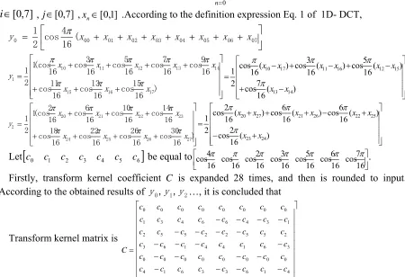
, j[0,7] ,x_n[0,1] .According to the definition expression Eq. 1 of 1D- DCT,

      _ _ _ _ _ _ _

 00 01 02 03 04 05 06 07

0 ( 16 4 cos 2 1 x x x x x x x x y                      ) 16 15 cos 16 13 cos 16 11 cos 16 9 cos 16 7 cos 16 5 cos 16 3 cos 16 (cos 1 2 1 17 16 15 14 13 12 11 10 1 x x x x x x x x y                             ) ( 16 7 cos ) ( 16 5 cos ) ( 16 3 cos ) ( 16 cos 2 1 14 13 15 12 16 11 17 10 x x x x x x x x                         ) 16 30 cos 16 26 cos 16 22 cos 16 18 cos 16 14 cos 16 10 cos 16 6 cos 16 2 (cos 1 2 1 27 26 25 24 23 22 21 20 2 x x x x x x x x y                             ) ( 16 2 cos ) ( 16 6 cos ) ( 16 6 cos ) ( 16 2 cos 2 1 24 23 25 22 26 21 27 20 x x x x x x x x    

Let



c₀ c₁ c₂ c₃ c₄ c₅ c₆



be equal to

    16 7 cos 16 6 cos 16 5 cos 16 3 cos 16 2 cos 16 cos 16 4

cos       .

Firstly, transform kernel coefficient C is expanded 28 times, and then is rounded to input.

According to the obtained results of

y

0,

y

1,

y

2…, it is concluded that

Transform kernel matrix is

                                                       6 4 3 1 1 3 4 6 5 2 2 5 5 2 2 5 4 1 6 3 3 6 1 4 0 0 0 0 0 0 0 0 3 6 1 4 4 1 6 3 2 5 5 2 2 5 5 2 1 3 4 6 6 4 3 1 0 0 0 0 0 0 0 0 c c c c c c c c c c c c c c c c c c c c c c c c c c c c c c c c c c c c c c c c c c c c c c c c c c c c c c c c c c c c c c c c C

According to the derivation process of 1D-DCT and the symmetric characteristics of the transform

kernel matrix, T

XC

Y



can be expressed as:











































4 3 5 2 6 1 7 0 5 2 2 5 0 0 0 0 2 5 5 2 0 0 0 0 6 4 2 0 k k k k k k k k k k k k

x

c

y











































4 3 5 2 6 1 7 0 1 3 4 6 3 6 1 4 4 1 6 3 6 4 3 1 7 5 3 1 k k k k k k k k k k k k

x

c

y

[image:3.612.81.531.94.402.2]

The above optimization algorithm shows that the multiplication of the 8*8 matrix and the 8*1 vector can be replaced by the product of 4*4 matrix and 4*1 vector which is structural rules and can be parallel calculated. So the number of multipliers of the DCT algorithm is reduced by half. In order to offset the data expansion caused by the kernel coefficient C when inputting previous, ID-DCT post-processing operation is performed by ignoring the lower 8 bits and keeping the high bits of the result of the secondary adder .The high bit yields the correct result for the 1D-DCT operation. 1D-DCT simulation result based on Altera cyclone IV EP4CE40F17C8N is shown in figure 1:

Figure 1. 1D-DCT simulation based on FPGA.

Implementation of Matrix Transposition

(4)

transform. In matrix transposition, there are no other operations, such as multiply, add, etc., but shifting mainly. Considering to promote the speed of the 2D-DCT algorithm, it is necessary that when transpose memory RAM receives the output data of the first level ID-DCT transformation, at the same time transpose memory RAM must be able to provide the second level 1D-DCT with the input data. So it ensures that the front and rear 1D-DCT can work continuously to improve the real-time performance of system. Here we adopt dual-RAM structure that ping-pong works, that is, two RAM blocks work alternately in the read / write mode. Each RAM has 64 memory cells, 6 address lines. When Writing data, let the RAM write- address be wr_cnt [5: 0].When reading data, let the RAM read-address be rd_cnt [5: 0], where rd_cnt [5: 3] is the row address after transposition and rd_cnt [2 : 0] is the column address after transposition.

Implementation of 2D-DCT

The second-level ID-DCT method is the same as the first-level 1D-DCT by and large. In order to prevent the overflow of data, the data width is changed from 8 bits to 12 bits to complete the second level DCT operation. Obtaining the high bits of output data of the second level 1D-DCT operation is the final 2D-DCT results. The 2D-DCT result of the 8 * 8 matrix sub-block( expression (5)) is as follows:

          

 

          

 

   

  



  

 



 

  

 



 

 

2 4 1 3 2 0 1 1

5 3 3 1 1 2 2 2

2 14 7 4 3 8 9 5

6 5 3 2 9 8 3 6

2 5 10 15 4 5 11 8

2 5 9 15 1 1 5 12

5 14 3 5 13 11 25 34

6 1 1 10 19 2 49 217

T

CXC Z

From the result of 2D-DCT of the 8 * 8 matrix sub-block image, it can be seen that the values are concentrated in the upper left corner and the values of the lower right corner is very small after 2D-DCT, because of large correlation between the source data of the image pixel. After normalized processing, the lower right corner will generally be zero. This is the physical meaning of DCT in image processing which the redundant space in transform domain is eliminated.

MATLAB Simulation of the 2D-DCT Algorithm

2D-DCT MATLAB simulation program code is as follows: Clear;

Clc;



X [40,33,33,22,26,40,36,26;43,26,33,22,29,43,22,36;36,33,29,26,15,33,26,4;36,43,26,33,

29,29,19,4;43,40,19,36,36,33,15,26;33,33,33,26,22,29,26,12;33,40,29,26,33,12,12,4;26,33,29,22,12 ,4,8,0];

C=zeros(8,8);

For i=0:7 For j=0:7 If i==0 b=sqrt( 4 2_);

Else b=sqrt(

4 1_);

End

C(i+1,j+1)=b*cos(pi*(j+0.5)*i/4);

End End

'

CXC

(5)



ZZ det2(X );

The result of the program operation is:

          

 

          

 

   



  



  

 

  

 



 

 

494 . 2 073 . 4 539 . 1 040 . 3 583 . 1 355 . 0 597 . 0 087 . 1

197 . 4 105 . 3 811 . 2 082 . 1 869 . 0 764 . 2 763 . 1 699 . 1

000 . 2 283 . 14 752 . 6 255 . 4 604 . 2 653 . 7 396 . 9 721 . 4

997 . 9 014 . 5 638 . 2 613 . 2 172 . 9 855 . 7 585 . 3 061 . 6

381 . 6 563 . 5 135 . 10 141 . 15 699 . 3 408 . 4 394 . 10 351 . 8

000 . 2 368 . 5 304 . 9 750 . 14 565 . 1 412 . 1 988 . 4 500 . 12

873 . 5 909 . 14 977 . 2 774 . 4 737 . 12 573 . 10 953 . 24 441 . 34

083 . 6 590 . 0 911 . 0 250 . 10 661 . 19 732 . 2 224 . 49 500 . 214

ZZ Z

It can be seen that the results of 2D-DCT based on FPGA is basically the same as the result of det2 function calculation in matlab. The error comes from intercepting the high bits in the fixed-point operation of FPGA and ignoring the low bits data. The correctness of the 2D-DCT algorithm based on FPGA is verified.

Summary

We discuss the sparse transform of image in CS theory, focus on the sparse method based on 2D-DCT orthogonal basis and row-column decomposition in FPGA. This method adopts two levels 1D- DCT series to achieve2D-DCT of the image and the row and column conversion intermediate matrix Y is embedded between two ID- DCT. The rationality of the algorithm is verified by the comparison between the results of the 2D-DCT based on FPGA and the results in MATLAB. Here the width of the data is enlarged, the high bits is intercepted, and ignoring low bits method is used to prevent the fixed-point data from overflowing. In the future, we try to use custom floating point numbers in the data processing.

Acknowledgements

The authors would like to thank their colleagues and family help and support in the study. This research was financially supported by the National Science Foundation and Province Science Foundation. The authors would like to thank The National Natural Science Foundation of China (NO. 61401356)) and the Natural Science Foundation Fund (NO. 2017JM6040) of Shaanxi Province, China for continual support.

References

[1] Qing Wang, Jia Li, Yi Shen."A Survey on Deterministic Measurement Matrix Construction Algorithms in Compressive Sensing [J]" Acta Electronica Sinica Vol 41, No.10 p. 2041-2050 (2013). [2] Hong-Peng Yin, Zhao-Dong Liu, Yi Chai. "Survey of Compressed Sensing [J]" Control and Decision, Vol 28, No.10, p. 1442-1453 (2013).

[3] Yue-Mei Ren, Yan-Ning Zhang, Ying Li. "Advances and Perspective on Compressed Sensing and Application on Image Processing [J]", Acta Automatica Sinica Vol 40, No.8, p. 1563-1575(2014).

[4] Xiao-Bo Qu, Di Guo, Ben-De Ning. "Undersampled MRI Reconstruction with the Patch-based Directional Wavelets [J]" Magnetic Resonance Imaging, Vol 30, No.7, p. 964-977 (2012).