Does the Food Stamp Program Really Increase Obesity? The Importance of Accounting for Misclassification Errors

Munich Personal RePEc Archive

Does the Food Stamp Program Really

Increase Obesity? The Importance of

Accounting for Misclassification Errors

Vassilopoulos, Achilleas and Drichoutis, Andreas and Nayga,

Rodolfo and Lazaridis, Panagiotis

Agricultural University of Athens, University of Ioannina, University

of Arkansas

January 2011

Online at

https://mpra.ub.uni-muenchen.de/41811/

Does the Food Stamp Program Really Increase Obesity?

The Importance of Accounting for Misclassification Errors

Achilleas Vassilopoulos1,Andreas C. Drichoutis2, Rodolfo M. Nayga, Jr.3and

Panagiotis Lazaridis4

1

Dept. of Agricultural Economics and Rural Development, Agricultural University of

Athens, Greece, email: avas(at)aua.gr

2 _{Dept. of Economics, University of Ioannina, Greece, email: adrihout(at)cc.uoi.gr}

3

Dept. of Agricultural Economics and Agribusiness, University of Arkansas, USA;

Norwegian Agricultural Economics Research Institute. email: rnayga(at)uark.edu

4 _{Department of Agricultural Economics and Rural Development, Agricultural}

University of Athens, Greece, email: t.lazaridis(at)aua.gr

Abstract

Over the last few decades, the prevalence of obesity among US citizens has grown

rapidly, especially among low-income individuals. This has led to questions about the

effectiveness of nutritional assistance programs such as the Supplemental Nutrition

Assistance Program (SNAP), formerly known as the Food Stamps Program (FSP).

Results from previous studies generally suggest that FSP participation increases

obesity. This finding is however based on the assumption that participants do not

misclassify their program participation despite significant misclassification errors

reported in the literature. Using propensity score matching and a new method to

conduct extensive sensitivity analysis, we conclude that this finding is sensitive to

misclassification errors above 10% and to the conditional independence assumption.

JEL codes:C63, D12, I1

2

1. Introduction

Obesity is increasing worldwide in dramatic rates. The World Health Organization

indicated that there were 1.4 billion overweight adults and at least 500 million obese

adults in the world in 2008 (WHO (2012) Obesity and Overweight. Fact Sheet No 311.

World Health Organization). By 2015, these figures are expected to rise to 2.3 billion

overweight and 700 million obese adults. Obesity effects on health are well supported

by the medical literature and include a long non-exhaustive list that includes

osteoarthritis, sleep apnea, asthma, high blood pressure, gallbladder disease,

cholesterol, type II diabetes, cardiovascular disease, stroke, renal and genitourinary

diseases (Bray, 2004, Esposito et al., 2004, Grundy, 2004, Whitmer et al., 2005,

Ejerblad et al., 2006, Van der Steeg et al., 2007). Obesity may also inflict severe

emotional harm, such as social stigmatization, depression, and poor body image.

Researchers have rightly responded to this unprecedented rise of obesity as

evidenced by the exploding number of papers published in the nutrition/medical as

well as the economics literature. The economic causes of obesity for adults and

children are nicely analyzed in Rosin (2008) and Papoutsi et al (2012), respectively.

Among the many factors linked to the high obesity prevalence are the increased

opportunity cost of time for food preparation, along with the availability of “cheap”

calories provided by fast-food restaurants, as well as the adoption of sedentary

lifestyles (Cutler et al., 2003, Philipson and Posner, 2003, Lakdawalla et al., 2005).

One interesting aspect of the obesity epidemic is that prevalence rates have been

found to be higher and to increase more rapidly among lower income people, a group

usually associated with fewer resources and poor diets.

To this respect, a number of nutrition assistance programs funded by the U.S.

3

andnutrition concerns. The Supplemental Nutrition Assistance Program (SNAP),

formerly known as the Food Stamps Program (FSP)1 is by far the largest nutrition

assistance program in the US. The FSP as implemented in 1964 was designed to

alleviate hunger by distributing coupons that could only be used to purchase food at

grocery stores. FSP benefits are given to a single person or family who meets the

program’s requirements pertaining to income, assets, work and immigration status.

Most benefit periods last for 6 months but some can be as short as 1 month or as long

as 3 years. Currently, electronic benefit transfers that operate essentially as debit cards

have replaced food stamp coupons. According to USDA data, about 40 million

individuals and 18 million households nation-wide participate in this program, with

total amount of benefits reaching 65 billion USD in 2010. Eligibility and benefits are

based on household size, household assets, and income. Other food assistance

programs in the US include the School Breakfast Program (SBP), the National School

Lunch Program(NSLP) andthe Women, Infant and Children Program (WIC).

Due to increasing obesity rates in the US, particularly among low-income

individuals, this paper is focused on assessing the effect of FSP on obesity. There are

two main theories on how food stamp benefits could contribute to weight gain: (1)

food stamps encourage beneficiaries to spend more money on food than they

otherwise would (and presumably, to eat more); and (2) food stamp participation is

linked to a cycle of deprivation followed by abundance and binge eating, which

results in weight gain over time (Ver Ploeg et al., 2007).

Several studies have examined the effect of FSP participation on various

outcomes. These studies differ in terms of the targeted groups (e.g., children, adult

1 _{For the rest of the paper we use the term FSP rather than SNAP since this program is still more popularly known}

4

women/men and the elderly), the outcomes of interest (e.g., Body Mass Index, food

security index, probability of being overweight/obese), the nature (e.g.,

cross-sectional, longitudinal) and the sources of the data2 as well as the methodology they

employ3. Results from a number of past studies suggest a positive effect of FSP

participation on adult obesity. For example, Baum (2007) found that FSP participation

increases the probability of being obese in females aged 20-28 while the amount of

food stamps benefit was positively related to BMI in males of the same age group.

Gibson(2003) concluded that FSP participation is responsible for a 2 percentage point

increase in the BMI of adult women. This effect was even greater in the case of

long-term participation. Chen et al. (2005) also found that women FSP beneficiaries have

an obesity rate that is 6.7 percent higher than that of women non- beneficiaries. On

the other hand, Kaushal (2007) found no significant effect of FSP participation on

obesity of both men and women.

These past studies, however, did not take into account the misclassification

errors associated with self-reported FSP participation status. This issue is important

since results could be sensitive to these misclassification errors, which have been

reported in the literature to be non-trivial. For instance, Bollinger and David (1997)

and Bitler et al. (2003) suggest that about 10%-15% of recipients do not report FSP

participation when asked by the interviewer while Meyer et al. (2010) report an even

higher (35%-50%) misclassification error. If this is the case, then previous findings

2

The Panel Study of Income Dynamics (PSID) along with the Child Development Supplement (CDS), the

National Health and Nutrition Examination Survey (NHANES), the National Longitudinal Survey of Youth

(NLSY79), the Health and Retirement Study (HRS) and the Asset and Health Dynamics Among the Old (AHEAD)

are some of them.

3 _{Descriptive statistics, OLS and Logistic Regressions, IV estimators (with and without fixed effects), Bivariate}

5

associating FSP participation with obesity could be biased and misleading. Our

objective is to assess how misclassification errors could affect the estimated effects of

FSP participation on obesity. We also take into account the complex endogeneity

issues inherent in these types of analysis and extensively assess the robustness of our

results to deviations from the usual assumptions.

Since FSP participation is not randomly but rather endogenously assigned to

subjects according to some observable (e.g., eligibility criteria) and unobservable (e.g.,

information acquisition, attitudes etc.) factors, it is very likely that some of these

factors are highly correlated with the outcome of interest, making it hard to uncover

any causal effect without a proper identification strategy. In this study, we employ the

propensity score matching method and perform an extensive sensitivity analysis to

assess the robustness of its restrictive assumptions. Quoting Angrist and Pischke

(2010), scrutinizing our results through a sensitivity analysis process is what takes the

con out of the econometrics.

We build on the work of Ichino et al.(2008) who proposed an excellent way of

assessing the robustness of matching estimators while avoiding parametric

assumptions. We then extend this method to account for the misclassification errors in

FSP participation. To our knowledge, this is the first time such a sensitivity analysis is

performed in the literature. To illustrate how misclassification errors could affect the

estimated effects of FSP participation on obesity, we utilize the 2005–2006 National

Health and Nutrition Examination Survey (NHANES). NHANES is designed to

assess the health and nutritional status of adults and children in the US and is unique

in that it combines interviews and physical examinations.

2. Methods

6

The research question of interest is whether participating in the FSP increases

the probability of being obese. Formally, assume that there is a binary indicator Y

that takes the value of 1 if the respondent has both a BMI4 greater than 30 kg/m2 and

a waste circumference (WC) greater than 100 cm, and 0 otherwise5. Define a second

binary variable T, indicating the treatment and being equal to 1 for participants and 0

for non-participants. Of course, a mere comparison of the obesity rate among

participants and non-participants does not reveal a causal relationship between the

FSP participationand obesity. It is likely that the two groups differ in many other

characteristics that could lead to differences in the outcome even if food stamps were

not received by either group. We postulate the existence of two potential binary

outcomes denoted by Y

 

 

and 0 otherwise and denote the outcome that would be realized in the case of

participation and non-participation respectively. It is obvious that we either observe

 

Y or Y

 

defined as:

(1) (0)

tY Y (1)

This effect, averaged over participants is the average treatment effect on the treated

(ATT) estimand, namely:

 







 



ATT E Y T  E Y T  (2)

4

The BMI (Body Mass Index) is used to define nutritional status and is derived from the division of Weight in kilograms by the square of height in meters. The acceptable range is the same for men and women and lies between 20 and 25. Obesity is taken to start at a BMI of 30 and gross obesity at 40. A BMI of 18-20 is defined as mild starvation and severe starvation begins when BMI falls below 16.

5

7

Since E Y( (0) |T 1) is not observed, one needs to make some additional

assumptions in order to estimate the ATT. The first is that Y(0), conditional on a set

of observable covariates X , does not influence participation in the program:

 

Y T X (3)

This assumption is widely known as the Conditional Independence Assumption (CIA),

the restrictive nature of which seems unappealing to many researchers and decreases

the popularity of matching estimators. A second assumption is the common support or

overlap condition, which ensures that for every FSP participant, there are

non-participants with the same observable covariates, that is:





Pr T 1 |X 1 (4)

In the estimations to follow, we ensure that observations falling out of the

common support region are excluded. If assumptions (3) and (4) hold, then after

conditioning on X , ATT becomes estimable through (2) by substituting the

unobservableE Y[ (0) |T 1,X], with its observable counterpart, E Y[ (0) |T 0,X]. To

solve the dimensionality problem arising when Xis a lengthy vector, Rosenbaum and

Rubin (1983) suggested the use of the propensity scoree X( ) Pr(T 1 |X), instead

of Xas the conditioning variable. Thus, the ATT parameter is given by:

 







 



{ 1} 1 | 1, ( ) 0 | 0, ( )

PSM T

ATT E _{ }E Y T  e X E Y T  e X _ (5)

Inasmuch as the FSP is designed to help low-income groups, it seems

reasonable that the control group should be the eligible non-recipients, classified as

such using the most important eligibility criterion of FSP participation, the Poverty

Income Ratio (PIR). The PIR is also the only available eligibility criterion in our

8

could render CIA implausible) are less likely to differ among individuals of these two

groups.

ATT can be estimated using several matching algorithms such as the nearest

neighbor, kernel, stratification, radius and spline smoothing. We use the nearest

neighbor propensity score matching, using the four nearest neighbors6 and report

analytical standard errors since the bootstrap variance estimator is invalid for nearest

neighbor matching (Abadie and Imbens, 2006). The variables used in the probit

regression in order to estimate the propensity score (e X( )) are shown in Table 1. The

first two variables are the outcome and the control variable respectively. In selecting

the variables to be included in the propensity score estimation we rely on the advice

of Rubin and Thomas (1996) and the evidence provided by Brookhart et al. (2006)

that one should include in the estimation of propensity scores all variables that are

thought to be related to the outcome, regardless of whether they are related to the

exposure. Household’s FSP participation (FS_hh) was used instead of the individual’s

participation status since FSP benefits are most certainly shared among the members

of the household. For the same reason, WIC participation (WIC_hh) was included in

the set of covariates. Other factors such as Alcohol and Smoker were included to

account for the non-food expenses of the groups which could reduce available

resources for food and decrease or increase the probability of being obese. Chronic

and DocDiab are used to account for the possible links between these different

6

When selecting the number of matches one has to consider the bias-variance trade-off, since utilizing multiple

matches for each treated individual will generally increase bias (2nd, 3rd, and 4th closest matches are, by

definition, farther away from the treated individual than is the 1st closest match) while on the other hand, it can

decrease variance due to the larger matched sample size (Stuart, 2010). We use four matches in order not to rely on

too little information but to also avoid incorporating observations that are not sufficiently similar. Like all

9

conditions and obesity. Square, cubic and interaction terms for all continuous

variables and their transformations were also included in the model. Millimet and

Tchernis (2009) showed that over-specifying the model used to estimate the

propensity score is always the best strategy, considering the penalty associated with

the under-specification. Finally, we include demographic variables such as age, ethnic

characteristics, educational level, income, marital status, and household size to

capture the biological differences affecting BMI, the awareness about nutrition issues

as well as the within-household consumption dynamics in the allocation of resources.

The estimates of ATT derived from the above procedure will be referred to as the

Unconfounded Baseline Estimates (UBEs). These are then compared with those

described below.

2.2. Misclassification errors

Due to the self-reported nature of the FSP participation data at hand, (5) is not

estimable, since what we observe is not Tbut T_obs. The difference between the two

indicators depends on whether the individuals that stated non-participation in FSP

were actually non-recipients or not7. Given that there is no way to identify those who

made a false-statement, the misclassification of subjects in the treated and the control

groups would have caused a severe bias through e X( ), thereby making the results

completely uninformative. Since some individuals are erroneously misclassified as

樂丹怒寧怜琉猪 ٻ ڈ ژ ک ہ ھ

underestimated depending on the extent of misclassification (see Battistin and Sianesi

2011). In addition, the ATT estimated from raw data could refer to a population

7

Although we ignore the proportion of individuals acting the other way around (i.e., reporting being FSP

participants while they are not) due to the fact that it is usually a negligible group, the proposed methodology can

10

different from the population the true ATT refers to, as some of the individuals with

1

T  _{might be discarded from the analysis due to violation of the common support or}

overlap condition. Finally, in the estimation with a confounder (analyzed in the next

section) there would be no possible way to define the parameters Pr_ijthat characterize

its distribution, since actual i’s are not known.

We circumvent this problem by simulating different scenarios where a

respondent that reported not to have received food stamps belies her true state of

participation by some probabilityPr





form assumptions about the probability distribution, we assume different

misclassification values in an attempt to discover a cut-off point, beyond which our

results fall flat. Specifically, we assess the robustness of our results to

misclassification errors of 5%, 10%, 15%, 20%, and 25% to cover the possible

misclassification errors suggested by Bollinger and David (1997), Bitler et al. (2003),

and Meyer et al. (2010). To accomplish this, we created m new databases9 for each

level of misclassification errors (i.e., 5m in total), with each of these datasets

containing all the variables that are exactly as in the original database and a new

participation indicator (FS_hh_new). The values of this dummy are same as those of

FS_hh, with the only difference being that a random10 percentage of zeroes (5%-25%

depending on the level of misclassification error examined) in the latter (FS_hh), are

8

Note that these values can be further decomposed into Pr









has strong evidence or a meaningful explanation on why the probability of misclassification can be related to the

outcome of interest.

9

In particular we've usedm=1000 but we keep this notation for demonstration simplicity.

11

transformed into ones in the former (FS_hh_new). Hence, we consider 5%-25% of the

non-participation reports to be false-statements.

It should be mentioned that during the simulation, from the whole pool of

possible datasets we utilize only those that satisfied the following criteria: a) the

averages of the covariates in the treated group and the weighted averages of the same

covariates in the control group were not to be significantly different11 based on a

Hotelling’s test, b) the probit model to be used for the estimation of the propensity

score passed a link test (Pedigon, 1980) and the Hosmer–Lemeshow (2000) goodness

of fit test with 10 groups, and finally c) after matching, all covariates in the probit

model were jointly insignificant as indicated by a Likelihood Ratio test as in Sianesi

(2004). Datasets not satisfying one of the above criteria were discarded and the

process continued until m datasets were constructed. This way, the danger of

introducing severe bias into the model or violating the balancing property (i.e. having

the treated and control units have the same distribution of observable covariates) is

mitigated. We then proceeded by obtaining a point estimate of ATT for each of the

new databases (i.eATT_{k PSM},mis for k=1,...m). Although it is relatively easy to calculate

mis

PSM

ATT by averaging overall point estimates, the calculation of the standard errors is

less straightforward. Using Rubin's (1987) combination of repeated complete-data

variances, we calculate the standard errors as:

  1 

1

mis

PSM m

ATT

se V B

m

 

  _{ }

  (6)

11

We use weighted averages for the control group since we employ a 4 to 1 nearest neighbor matching. The

weights are the common normalized weights that were then used in the estimation of the 4 to 1 nearest neighbor

12

where 1 1

m

 _ 

 

 is the correction factor (correcting for the fact that m is finite),Vis the

average of the estimated variances associated with each of the m  ,mis k PSM

ATT :

 

1

1 m

k k

V V

m 





andBm is the variance among the m ATT_{k PSM},mis :

   2

1

1

( , )

1

m _mis

mis

k _{P M} PSM k

m ATT _S ATT

B

m 

 





For a large number of replications the statistic ( ) / mis PSM mis

PSM ATT seATT

ATT  is

approximately normal.

2.3 Confounders

Another possible pitfall of the methodology is the possible bias of ATT_PSM in

the case of a failure of the CIA, namely:

 

 

 

BIAS E Y_ T  e X _E Y_ T  e X _ (9)

The bias is minimized when e(X)0.5 _{(Black and Smith, 2004, Heckman}

and Navarro-Lozano, 2004). Hence, Black and Smith (2004) suggested to estimate the

PSM

ATT , within the ‘thick support’ region of the propensity score (i.e.,

 

0.33e X 0.66 ). However, if treatment effect varies with X , the estimated

parameter would deviate from the corresponding population parameter and thus might

not be very informative. We follow a different strategy instead: we assume that CIA

13

U .12 In the case of CIA failure, such confounders once added would impose CIA to

the model and consequently would transform (5) into:

 







 







{ 1} 1 | 1, ( , ) 1 | 0, ,

conf PSM T

ATT E _{ }E Y T  e X U E Y T  e X U _ (10)

We are particularly interested in assessing how the baseline estimates of (5)

would change with the addition of possible confounders U, in order to perform a

robustness check of our results. If the findings suggest that conditional on the

existence of such confounders a positive effect is still in place, then one can be more

confident of the interpretation of the results. According to Ichino et al. (2008), it is

preferable to avoid parametric assumptions about the simulated confounder. Different

hypotheses about the distribution of the confounding factorcould be simulated by

imposing the values of the parameters characterizing the distribution of U





Pr_ij Pr U 1|T i Y,  j X, i j, 

 

according to these parameters, and finally estimate ATT_{k PSM},conf n times for the same

distribution parameters13 (i.e., for k=1,...,n). For each simulated confounder, the

conf

PSM

ATT is the average of all ATT_{k PSM},conf and these results will henceforth be called the

Confounded Baseline Estimates (CBEs) which are to be compared with the UBEs.

The formulas for the calculation of the standard errors of the ATTconfPSM _{are those}

shown in (6)-(8), replacing the subscripts m with n and ATTmisPSM with  conf PSM

ATT .

In each of the n iterations, two logit models (two odds ratios) are fitted

(calculated). The first (Pr





12

If inferences based on the UBEs are robust in the presence of binary confounders, then this holds even if the true

ones are continuous (see Ichino et al. (2006), for a proof via Monte Carlo simulations).

13

14

a confounder would have on the odds of being obese in the case of no treatment

(outcome effect), while the second (Pr





relative importance of the hypothesized confounder on the participation probability

(selection effect). The odd ratios obtained from the above models are referred to as α

and ε respectively.

As a first simulation practice, we simulate a neutral confounder (i.e., a

confounder which has exactly a 50% chance to be 1 in all possible treatment/outcome

combinations) and the confounders that mimic the distribution of some of the

demographic variables (i.e., Male, Chronic, Educ1, Educ2, Educ3,MarStat1, MarStat2).

The results are shown in Tables 5, 6, and 7. Since these results are highly dependent

upon the selection of the covariates, we then search for the possible existence of

confounders that could determine a positiveATTPSM even in the absence of a true

causal relationship between T and Y. As shown in Ichino et al. (2006), such

‘dangerous’ confounders can be simulated by fixing the probability Pr(U = 1) and the

difference pr11 − pr10 at some predetermined values14 and then assigning positive

values15 to d= pr01 – pr00 and s= pr1. – pr0., wherepri. Pr





through α and ε,we are able to assess how strong the confounders generated in this

particular configuration of parameters should be in order to alter inferences based on

_PSM

ATT . If only very strong confounders are capable of doing so, the findings are

considered to be robust to CIA failures.

14

We have set the value of Pr(U = 1) to 0.3 and that of p11 − p10to 0. Since these quantities are not expected to

represent a real threat to the baseline estimate, the results remain qualitatively intact when considering different

values.

15

To do so, we used the Matlab codeavailable on the website http://www.tommasonannicini.eu , which returns all

15

2.4 Misclassification errors and Confounders

Up to this point, we have managed to assess the robustness of inferences based

on UBEs by assuming misclassification errors and confounding variables separately.

However, we have ignored the possibility of these two deviations coexisting in our

settings. Hence, we need a combination of the two procedures described above to

further assess the validity of our results. The combining rule is a nested imputation

approach as described in Shen (2000) and employed in Rubin (2003) and Harel

(2007). According to this procedure, in each of the m databases created for each level

of misclassification errors (as previously demonstrated under the Misclassification

errors section), we construct n confounders for each set of parameters prij as described

above in the estimation of ATTconfPSM. As a result we end up with m×n (i.e. 1 million)

ATT estimates for each level of misclassification errors and each confounder

examined, the average of which provides the Misclassified Confounded Estimates

(MCEs) ATTmis confPSM, . The calculation of the standard errors of  , mis conf PSM

ATT is now more

tedious since the variability comes from multiple sources and is calculated as:

 mis conf,  1 1  (1 1)

PSM n m

ATT

se V B B

n m

 

  _{ }  

  (11)

where(1 1)

n

 and (1 1)

m

 are the correction factors (correcting for the fact that m and

n are finite), Vis the average of the estimated variances associated with each of the

 ,

, mis conf i PSM

ATT for i=1,..,.m n :

 

1 1

1 m n

k j kj

V m

V

n  



16 _m

B is the between database variance:

  ,  , 1 2 1 , 1 1 ( ) 1

m _{mis conf mis conf}

m kj PSM PS

n

M k j

B ATT ATT

m  n 

 



 

and Bn the average between imputation variance:

  ,  ,

1 1

2

1

, ,

1 1 1

( )

1

n _{mis conf mis conf}

n k

m n

k j j

j PSM kj PSM

B ATT ATT

m  n  n 

 









For a large number of replications the statistic   ,

,

)

( / mis conf PSM mis conf

PSM ATT seATT

ATT 

approximates a normal distribution.

To sum up, the methodology of the paper consists of foursteps. First, we estimate

PSM

ATT using nearest neighbor propensity score matching, using the four nearest

neighbors while assuming that CIA holds and that Pr





of this procedure are the Unconfounded Baseline Estimates (UBEs). Second, we

simulate different misclassification scenarios and obtain the Misclassified Baseline

Estimates (MBEs) that are compared with the UBEs. Next, we derive the CBEs and

MCEs by augmenting the model used for UBEs and MBEs separately with a neutral

confounder (i.e., a confounder which has exactly 50% chance to be 1 in all possible

treatment/outcome combinations) and with confounders that mimic the distribution of

known demographic variables (Male, Chronic, Educ1, Educ2,

Educ3,MarStat1,MarStat2). In the final step, we generate confounders that could

incorrectly reveal a causal relationship between Y and T and assess the robustness of

our results to such 'dangerous' confounders using the CBEs and MCEs. In addition,

through α and ε, we are able to determine how strong the tolerance or sensitivity of

17

3. Data and Results

Researchers face additional problems when dealing with data on FSP participation

and weight outcomes. The first is that many US national surveys collect self-reported

data for weight and height which can render biased BMI values (Roberts, 1995, Hill

and Roberts, 1998). We circumvent this problem by using the 2005-06 National

Health and Nutrition Examination Survey (NHANES) which measures the weight and

height of individuals, thus reducing intentional and unintentional deviations from the

true values (i.e., measurement errors).

The 2005-2006 National Health and Nutrition Examination Survey (NHANES) is

designed to assess the health and nutritional status of adults and children in the United

States. The survey is unique in that it combines interviews and physical examinations

and includes demographic, socioeconomic, dietary, and health-related questions. The

examination component consists of medical, dental, and physiological measurements,

as well as laboratory tests administered by highly trained medical personnel. The

dataset includes 10,348 respondents in its fullest module.

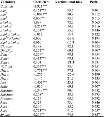
Results from the probit model used to estimate the propensity scores are given in

table 2, which also contains the percentage reduction of bias16 due to the matching

procedure as well as the probability of a type I error if we reject the null hypothesis of

noremaining bias after the matching. We offer a few remarks on these results. First,

we need to mention that we have not excluded the statistically insignificant covariates

in the construction of the propensity scores since our aim is to get the most

accurateestimation of that score and not of the model. Also, since no figure in the last

column is smaller than 0.10, we can accept the hypothesis of no remaining bias for all

18

variables used in the estimation of the propensity score at the 10% confidence level;

although for some covariates (e.gAge*Alcohol and Hsize2) the matching procedure

increased the bias between the treated and the control group. Finally, it is worth

noticing that the balancing property is satisfied within the five strata17 of the common

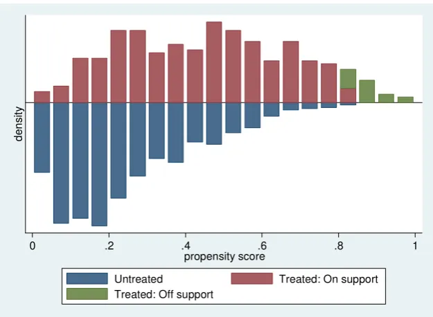
support region which is 0.004 to 0.833 while, as shown in Figure 1, there seems to be

large heterogeneity of the treated and control groups with respect to the propensity

score.

Figure 1. Propensity score (density of probability intervals by participation status)

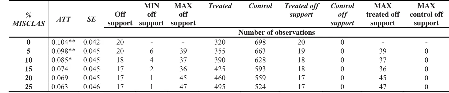
At a first glance in Table 3, one can notice that the UBEs show that FSP

participation increases the likelihood of being obese by 10.4%. As we move on to

Table 4 where the MBEs are presented for the five levels of misclassification errors18,

we can see that when 5% and 10% misclassification errors are examined, the effect of

the FSP on the likelihood of being obese still remains statistically significant at the

17

The optimal number of blocks was selected by the pscore procedure in Stata. 18

In the first line we also include the UBEs to facilitate comparisons. As a matter of fact, UBEs can be considered

a special case of MBE where the level of misclassification errors is 0%.

de

ns

it

y

0 .2 .4 .6 .8 1 propensity score

19

10% confidence level. However, if 15% or more of the participants have made a

false-statement about their participation status, theATTmisPSMsuggests that the causal effect

becomes questionable. Hence, the positive ATT is only robust to misclassification

errors of 10% or less.

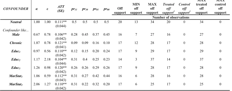
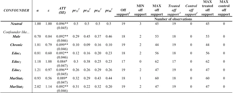
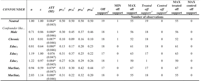
The CBEs and MCEs for potential confounders that mimic the distribution of

known covariates for 5% and 10% misclassification errors are exhibited in Tables 5, 6,

and 7. We only present the results on these two levels of misclassification errors since

in the previous step we found that for higher misclassification levels the ATT is not

robust even when the CIA holds. The CBEs show that when there are no

misclassification errors, the results are robust to the existence of confounders that

mimic the distribution of all selected covariates. From the values of α and ε, we also

conclude that the outcome and selection effects of such confounders are not very

strong. This is also true for the MCEs under the 5% misclassification errors. However,

when 10% misclassification errors are assumed, the ATT in the presence of some

confounders (those that mimic the distribution of Educ2, MarStat1) is not statistically

significant at the 10% confidence level.

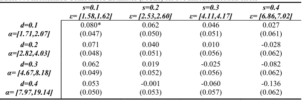
In Tables 8, 9 and 10, the CBEs and MCEs are also presented but this time with

confounders that are designed to carry all the properties of a ‘dangerous’ confounder.

As we move down each row in these tables, the selection effect (ε) is held constant

and the outcome effect (α) of the hypothesized unmeasured variable increases, whilst

the exact opposite is true when moving along each line. Moving down the first

column of Table 8, we find that for no misclassification errors, the result of a positive

effect of the FSP on the likelihood of being obese of the participants is very robust to

unobservable confounders with strong outcome effects; it is also relatively robust to

20

presence of an unobservable confounder, the selection effect is 1.58 to 1.6319; but for

the ATT to become not statistically significant, it should also have an outcome effect

of more than 7.3320. However, for unobservable confounders with higher selection

effects, the causal effect of the FSP could prove to be an artifact of the CIA, even for

weaker outcome effects. The same pattern is also observed for the 5%

misclassification errors (Table 9) but in this case the estimator appears to be also more

sensitive to the outcome effect of the possible confounder (although confounders with

such a high outcome effects are still rather strong). Finally, for 10% misclassification

errors (Table 10), the MCEs indicate that the treatment effect is very sensitive to

additional confounders since the ATT parameter is not statistically significant even

for small outcome/selection effects. Overall, the positive effect of FSP participation

on obesity for participants is very (quite) robust to the existence of confounders when

there is 0% (5%) misclassification errors. Hence, in these cases, we can claim that the

treatment effect is not an artifact of our assumptions. However, we cannot conclude

the same thing in the presence of 10% misclassification errors and some unobservable

confounder.

4. Concluding Remarks

The Food Stamp Program is one of the few nutritional assistance programs in the

history of the US that has drawn so much attention. Due to the high prevalence of

obesity among low-income individuals, a number of papers have examined the effect

of FSP participation on obesity. Most of these studies have suggested a positive effect.

19

Which in turn means that individuals for whom this confounder is equal to 1 are 58%-63% more likely to

participate in the FSP that the others.

20

Meaning that non participants for whom this confounder is equal to 1 are 633% more likely to be obese than

21

However, none of these studies has evaluated the potential effect of misclassification

errors (i.e., misreporting of actual participation status) in the analysis. We feel that

this is a very important issue since results could be sensitive to these misclassification

errors up to a point where findings can be considered no longer valid. In this study,

we examined the complex interrelationship of FSP participation and the likelihood of

being obese of participants using propensity score matching. We then assessed the

robustness of our results under different misclassification errors in the treatment

variable as well as the extent of the presence of additional confounders that would be

needed for the Conditional Independence Assumption to hold.

Our results suggest that participation in FSP is linked to a 10.4% higher

likelihood of being obese for adult participants. This result is robust to CIA but only

when misclassification errors are 10% or less. Hence, if the predictions of Bollinger

and David (1997) and Bitler et al. (2003) are accurate that about 10% to 15% of the

participants are misreporting their FSP participation status, then one should be more

cautious about the accuracy or validity of the causal effect of FSP participation on

obesity. Specifically, our results indicate that if the level of misclassification error is

above 10%, the ATT becomes extremely sensitive to plausible confounders. This

issue is important since it can even be possible that misclassification errors are

significantly greater than 15% according to Meyer et al. (2010). With

misclassification errors of 15% or more, our results reveal no statistically significant

effect even under CIA.

Our findings have significant implications for future analyses of FSP

participation effects since we provide credible evidencethat questions the positive

correlation between FSP and obesity suggested inprevious studies that failed to

22

our findings, failure to account for these potential sources of biases can render results

inaccurate and unreliable for policy making. Similar to the majority of previous

papers, a weakness of our study is the lack of information in our data about the

duration of participation in the program. Nevertheless, a critical implication of our

findings is that misreporting of self-reported participation information should also be

taken into account when analyzing the effect of duration of FSP participation on

health related outcomes. This would not be an issue with revealed or measured

23

Table 1. Names and descriptions of the variables

* These variables were dropped from estimations to avoid perfect multicollinearity Variables Description

Obese Dummy, respondent’s BMI≥30 kg/m2 & WC≥100 cm

FS_hh Dummy, household received food stamps last year

Age Age of respondent

Alcohol Average glasses (250 ml) of alcohol consumed by respondent the last 2 days

Chronic Dummy, Respondent suffers from coronary heart disease, heart attack, stroke or liver condition

DocDiab Dummy, Respondent has been diagnosed for diabetes/prodiabetes or at risk of diabetes

Educ1 Dummy, up to 9th grade

Educ2 Dummy, 9th-11th grade/High school grad/GED or

equivalent

Educ3 Dummy, Some College or Associate of Arts degree

Educ4* Dummy, College graduate or above

WIC_hh Dummy, household received Women, Infants and Children benefits last year

Hsize1 Dummy, Household size<2

Hsize2 Dummy, 2Household size<5

Hsize3 Dummy, 5Household size<7

Hsize4* Dummy, Household size7

Inc1 Dummy, Annual household income<$24,999

Inc2* Dummy, $25,000<Annual household Income<$54,999

Male Dummy, Respondent male

MarStat1 Dummy, Respondent married

MarStat2 Dummy, Respondent divorced/separated/widowed

MarStat3* Dummy, Respondent unmarried

Pregnant Dummy, Respondent was pregnant at examination

Race1 Dummy, Hispanic race

Race2 Dummy, Ethnicity is non-Hispanic White Race

Race3 Dummy, Ethnicity is non-Hispanic Black Race

Race4* Dummy, Other ethnicity

24

Table 2. Results of the propensity score (Probit) estimation

*,**,*** statistically significant at the 10%,5% and 1% level respectively

Variables Coefficient %reductionof bias Prob.

Constant -2.931***

Age 0.161*** 93.6 0.401

Age2 -0.003*** 90.9 0.512

Age3 0.000** 93.7 0.613

Alcohol 1.989 72.3 0.665

Alcohol2 -2.214** 54.2 0.516

Alcohol3 0.503** 55.0 0.436

Age* Alcohol -0.012 -0.7 0.322

Age2* Alcohol 0.000 -38.6 0.194

Age* Alcohol2 0.010 -15.3 0.304

Chronic 0.198 72.1 0.752

DocDiab 0.232** 69.1 0.707

Educ1* 0.259* 98.1 0.954

Educ2 0.413*** 98.1 0.954

Educ3 0.103 -81.3 0.681

WIC_hh 0.575*** 93.4 0.751

Hsize1 -0.771*** 97.1 0.904

Hsize2 -0.272 -25.6 0.199

Hsize3 -0.146 21.2 0.235

Inc2 -0.403*** 23.1 0.404

Male -0.036 69.1 0.707

MarStat1 -0.349*** 99.4 0.982

MarStat2 0.268* 58.6 0.773

Pregnant 0.119 68.5 0.592

Race1 0.124 93.4 0.846

Race2 0.249 85.2 0.732

Race3 0.723*** 91.5 0.657

25 Table 3. Unconfounded Baseline Estimates (UBEs)

ATT SE

p-value

OFF SUPPORT

TREATED CONTROL TREATED

OFF SUPPORT

CONTROL OFF SUPPORT Number of observations

0.104 0.042 0.01 20 320 698 20 0

Table 4. Misclassified Baseline Estimates (MBEs)

%

MISCLAS ATT SE

Off support

MIN off support

MAX off support

Treated Control Treated off

support

Control off support

MAX treated off

support

MAX control off

support Number of observations

0 0.104** 0.042 20 - - 320 698 20 0 - -

5 0.098** 0.045 20 6 39 355 663 19 0 39 0

10 0.085* 0.045 18 4 37 390 628 18 0 37 0

15 0.074 0.045 17 2 36 425 593 18 0 36 0

20 0.069 0.045 17 1 45 460 559 17 0 45 0

25 0.063 0.046 17 1 47 495 524 17 0 47 0

26 Table 5. Confounded Baseline Estimates (CBEs)

CONFOUNDER α ε ATT

(SE) pr11 pr10 pr01 pr00 Off

support

MIN off support

MAX off support

Treated off support1

Control off support1

MAX treated

off support

MAX control

off support Number of observations

Neutral 1.00 1.00 0.111** (0.044)

0.5 0.5 0.5 0.5 20 13 34 20 0 34 0

Confounder like...

Male 0.67 0.78 0.106** (0.042)

0.28 0.45 0.37 0.45 16 7 27 16 0 27 0

Chronic 1.87 0.78 0.121** (0.041)

0.09 0.09 0.16 0.10 17 12 28 17 0 28 0

Educ1 0.97 0.56 0.110** (0.042)

0.12 0.15 0.20 0.24 17 9 29 17 0 29 0

Educ2 1.17 2.18 0.104**

(0.044)

0.31 0.4 0.25 0.23 14 3 37 14 0 37 0

Educ3 1.26 0.98 0.120** (0.042)

0.26 0.26 0.29 0.26 17 9 28 17 0 28 0

MarStat1 1.06 0.59 0.112**

(0.043)

0.31 0.27 0.42 0.44 16 6 28 16 0 28 0

MarStat2 2.06 1.27 0.110** (0.042)

0.31 0.22 0.32 0.20 17 6 25 17 0 25 0

1

27

Table 6.Misclassified Confounded Estimates (MCEs) for 5% misclassification errors

CONFOUNDER α ε ATT

(SE) pr11 1

pr101 pr011 pr001 Off

support2 MIN off support MAX off support Treated off support 2

Control off support2 MAX treated off support MAX control off support Number of observations

Neutral 1.00 1.00 0.096** (0.045)

0.5 0.5 0.5 0.5 19 3 45 19 0 45 0

Confounder like...

Male 0.70 0.84 0.092** (0.046)

0.29 0.45 0.37 0.46 18 2 53 18 0 53 0

Chronic 1.81 0.79 0.099** (0.046)

0.10 0.09 0.16 0.10 19 2 44 19 0 44 0

Educ1 0.81 0.60 0.092** (0.046)

0.12 0.16 0.20 0.23 18 2 56 18 0 56 0

Educ2 1.18 1.88 0.084* (0.047)

0.3 0.38 0.25 0.23 17 0 62 17 0 62 0

Educ3 1.21 0.97 0.096** (0.045)

0.26 0.26 0.29 0.26 19 2 47 19 0 47 0

MarStat1 0.93 0.56 0.089*

(0.047)

0.32 0.29 0.43 0.44 18 1 60 18 0 60 0

MarStat2 2.02 1.14 0.092** (0.046)

0.31 0.22 0.32 0.20 19 2 47 19 0 47 0

1

These are average percentages over all simulations since the value of the distribution parameters of the demographic variables on the treatment/outcome condition were different in each of the 1,000 simulated databases.

2

28

Table 7. Misclassified Confounded Estimates (MCEs) for 10% misclassification errors

CONFOUNDER α ε ATT

(SE) pr11 1

pr101 pr011 pr001 Off

support2 MIN off support MAX off support Treated off support 2

Control off support2 MAX treated off support MAX control off support Number of observations

Neutral 1.00 1.00 0.084* (0.043)

0.50 0.50 0.50 0.50 19 1 55 19 0 55 0

Confounder like...

Male 0.71 0.86 0.080* (0.046)

0.30 0.45 0.37 0.46 18 1 56 18 0 56 0

Chronic 1.81 0.81 0.087* (0.046)

0.10 0.09 0.16 0.10 18 1 52 18 0 52 0

Educ1 0.81 0.64 0.080* (0.046)

0.13 0.17 0.20 0.23 18 0 61 18 0 61 0

Educ2 1.19 1.80 0.076 (0.047)

0.31 0.37 0.25 0.22 17 0 63 17 0 63 0

Educ3 1.22 0.97 0.084* (0.045)

0.27 0.26 0.29 0.26 18 1 50 1 0 50 0

MarStat1 0.94 0.59 0.079*

(0.047)

0.33 0.30 0.42 0.44 17 0 67 17 0 67 0

MarStat2 2.03 1.14 0.080* (0.046)

0.31 0.22 0.32 0.20 18 0 55 18 0 55 0

1

These are average percentages over all simulations since the value of the distribution parameters of the demographic variables on the treatment/outcome condition were different in each of the 1,000 simulated databases.

2

29 Table 8. Confounded Baseline Estimates (CBEs)1

s=0.1 ε= [1.58,2.60]

s=0.2 ε= [2.57,2.60]

s=0.3 ε= [4.11,4.19]

s=0.4 ε= [6.82,6.94] d=0.1 α=[1.70,2.03] 0.091* (0.048) 0.070 (0 .051) 0.057 (0 .055) 0.037 (0.062) d=0.2

α=[1.71,3.86] (0 .048) 0.090*

0.046 (0 .052) 0.020 (0.057) -0.017 (0.063) d=0.3 α= [4.70,7.66]

0.071 (0 .050) 0.025 (0.053) -0.018 (0.057) -0.069 (0.063) d=0.4 α= [7.95,11.68]

0.063 (0.051) 0.004 (0.054) -0.052 (0.059) -0.124 (0.064) 1

For each of these 16 models, similar results such as those in Tables 5-7 are available upon request * Statistically significant at the 10% level

Table 9. Misclassified Confounded Estimates (MCEs) for 5% misclassification errors1

s=0.1

ε= [1.58,1.62] ε= [2.53,2.60] s=0.2 ε= [4.11,4.17] s=0.3 ε= [6.86,7.02] s=0.4 d=0.1 α=[1.71,2.07] 0.080* (0.047) 0.062 (0.050) 0.046 (0.051) 0.027 (0.061) d=0.2

α=[2.82,4.03] (0.048) 0.071

0.040 (0.051) 0.010 (0.056) -0.028 (0.062) d=0.3

α= [4.67,8.18] (0.049) 0.062

0.019 (0.052) -0.025 (0.056) -0.082 (0.062) d=0.4 α= [7.97,19.14]

0.053 (0.050) -0.001 (0.053) -0.060 (0.057) -0.136 (0.062) 1

For each of these 16 models, similar results such as those in Tables 5-7 are available upon request. * Statistically significant at the 10% level

Table10.Misclassified Confounded Estimates (MCEs) for 10% misclassification errors1

s=0.1 ε= [1.62,1.63]

s=0.2 ε= [2.64,2.65]

s=0.3 ε= [4.37,4.39]

s=0.4 ε= [7.59,7.61] d=0.1 α=[1.73,2.24] 0.069 (0.047) 0.052 (0 .050) 0.035 (0 .054) 0.012 (0.061) d=0.2

α=[2.87,4.76] (0 .048) 0.059

0.030 (0 .051) -0.004 (0.055) -0.051 (0.061) d=0.3 α= [4.82,11.07]

0.050 (0 .048) 0.007 (0.052) -0.043 (0.056) -0.11 (0.062) d=0.4 α= [8.38,37.15]

0.040 (0.049) -0.015 (0.052) -0.082 (0.056) -0.176 (0.060) 1

30

References

Abadie A, Drukker D, Herr JL, Imbens GW. 2004. Implementing Matching

Estimators for Average Treatment Effects in Stata. Stata Journal 4: 290-311.

Abadie A, Imbens GW. 2006. Large Sample Properties of Matching Estimators for

Average Treatment Effects. Econometrica 74(1): 235-267.

Angrist J, Pischke J-S. (2010). The Credibility Revolution in Empirical Economics:

How Better Research Design Is Taking the Con out of Econometrics, National

Bureau of Economic Research.

Baum C. (2007). The Effects of Food Stamps on Obesity,The United States

Department of Agriculture (USDA), Economic Research Service (ERS).

Bitler MP, Currie J, Scholz JK. 2003. Wic Eligibility and Participation. Journal of

Human Resources 38: 1139-1179.

Black DA, Smith JA. 2004. How Robust Is the Evidence on the Effects of College

Quality? Evidence from Matching. Journal of Econometrics 121(1-2): 99-124.

Bollinger CR, David MH. 1997. Modeling Discrete Choice with Response Error:

Food Stamp Participation. Journal of the American Statistical Association 92

(439): 827-835.

Bray GA. 2004. Medical Consequences of Obesity. Journal of Clinical

Endocrinology & Metabolism 89(6): 2583-2589. 10.1210/jc.2004-0535

Brookhart MA, Schneeweiss S, Rothman KJ, Glynn RJ, Avorn J, Stürmer T. 2006.

Variable Selection for Propensity Score Models. American journal of

epidemiology 163(12): 1149-1156.

Chen Z, Yen ST, Eastwood DB. 2005. Effects of Food Stamp Participation on Body

Weight and Obesity. American Journal of Agricultural Economics 87(5):

31

Cutler DM, Glaeser EL, Shapiro JM. 2003. Why Have Americans Become More

Obese? Journal of Economic Perspectives 17(3): 93-118.

Ejerblad E, Fored CM, Lindblad P, Fryzek J, McLaughlin JK, Nyren O. 2006. Obesity

and Risk for Chronic Renal Failure. Journal of the American Society of

Nephrology 17(6): 1695-1702. 10.1681/asn.2005060638

Esposito K, Giugliano F, Di Palo C, Giugliano G, Marfella R, D'Andrea F,

D'Armiento M, Giugliano D. 2004. Effect of Lifestyle Changes on Erectile

Dysfunction in Obese Men: A Randomized Controlled Trial. Journal of the

American Medical Association 291(24): 2978-2984.

Gibson D. 2003. Food Stamp Program Participation Is Positively Related to Obesity

in Low Income Women. Journal of Nutrition 133(7): 2225-2231.

Grundy SM. 2004. Obesity, Metabolic Syndrome, and Cardiovascular Disease.

Journal of Clinical Endocrinology & Metabolism 89(6): 2595-2600.

10.1210/jc.2004-0372

Harel O. 2007. Inferences on Missing Information under Multiple Imputation and

Two-Stage Multiple Imputation. Statistical Methodology 4(1): 75-89.

Heckman J, Navarro-Lozano S. 2004. Using Matching, Instrumental Variables, and

Control Functions to Estimate Economic Choice Models. Review of

Economics and Statistics 86(1): 30-57.

Hill A, Roberts J. 1998. Body Mass Index: A Comparison between Self-Reported and

Measured Height and Weight. Journal of Public Health 20(2): 206-210.

Ichino A, Mealli F, Nannicini T. 2006. From Temporary Help Jobs to Permanent

Employment: What Can We Learn from Matching Estimators and Their

32

Ichino A, Mealli F, Nannicini T. 2008. From Temporary Help Jobs to Permanent

Employment: What Can We Learn from Matching Estimators and Their

Sensitivity? Journal of Applied Econometrics 23(3): 305-327.

Kaushal N. 2007. Do Food Stamps Cause Obesity? Evidence from Immigrant

Experience. Journal of Health Economics 26(5): 968-991.

Lakdawalla D, Philipson T, Bhattacharya J. 2005. Welfare-Enhancing Technological

Change and the Growth of Obesity. American Economic Review 95(2):

253-257.

Meyer BD, Goerge R, Hall C. (2010). The Analysis of Food Stamp Program

Participation with Matched Administrative and Survey Data,University of

Chicago Working Paper.

Millimet DL, Tchernis R. 2009. On the Specification of Propensity Scores: With

Applications to the Analysis of Trade Policies. Journal of Business &

Economic Statistics 27: 397-415.

Philipson TJ, Posner RA. 2003. The Long-Run Growth in Obesity as a Function of

Technological Change. Perspectives in Biology and Medicine 46.

Papoutsi GS, Drichoutis AC, Nayga JRM. 2012. The Causes of Childhood Obesity: A

Survey. Journal of Economic Surveys: 10.1111/j.1467-6419.2011.00717.x

Roberts RJ. 1995. Can Self-Reported Data Accurately Describe the Prevalence of

Overweight? Public Health 109(4): 275-284.

Rosenbaum PR, Rubin DB. 1983. The Central Role of the Propensity Score in

Observational Studies for Causal Effects. Biometrika 70(1): 41-55.

Rosenbaum PR, Rubin DB. 1985. Constructing a Control Group Using Multivariate

Matched Sampling Methods That Incorporate the Propensity Score. American

33

Rosin O. 2008. The Economic Causes of Obesity: A Survey. Journal of Economic

Surveys 22(4): 617-647.

Rubin DB. 1987. Multiple Imputation for Nonresponse in Surveys. New York, NY:

John Wiley and Sons.

Rubin DB. 2003. Nested Multiple Imputation of Nmes Via Partially Incompatible

Mcmc. Statistica Neerlandica 57(1): 3-18.

Rubin DB, Thomas N. 1996. Matching Using Estimated Propensity Scores: Relating

Theory to Practice. Biometrics 52(1): 249-264.

Shen Z. (2000). Nested Multiple Imputation,Cambridge, MA: Harvard University.

Stuart EA. 2010. Matching Methods for Causal Inference: A Review and a Look

Forward. Forthcoming in Statistical Science.

Van der Steeg JW, Steures P, Eijkemans MJC, Habbema JDF, Hompes PGA,

Burggraaff JM, Oosterhuis GJE, Bossuyt PMM, van der Veen F, Mol BWJ.

2007. Obesity Affects Spontaneous Pregnancy Chances in Subfertile,

Ovulatory Women. Human Reproduction 23(2): 324-328.

Ver Ploeg M, Mancino L, Lin B-H, Michele Ver Ploeg LM, Lin. (2007). Food and

Nutrition Assistance Programs and Obesity: 1976-2002,USDA.

Whitmer RA, Gunderson EP, Barrett-Connor E, Quesenberry CP, Yaffe K. 2005.

Obesity in Middle Age and Future Risk of Dementia: A 27 Year Longitudinal