Relationship between inflation and economic growth in Azerbaijani economy: is there any threshold effect?

Munich Personal RePEc Archive

Relationship between inflation and

economic growth in Azerbaijani

economy: is there any threshold effect?

Hasanov, Fakhri

Institute for Scientific Research on Economic Reforms, Ministry of

Economic Development of the Republic of Azerbaijan

June 2011

Online at

https://mpra.ub.uni-muenchen.de/33494/

Relationship between inflation and economic growth in Azerbaijani economy: Is there any threshold effect?

Fakhri Hasanov

Institute for Scientific Research on Economic Reforms, Ministry of Economic Development. AZ1011, H.Zardabi Avenue 88A, Baku, Azerbaijan.

Department of Modeling Socio-Economic Processes, Cybernetics Institute, Azerbaijan National Academy of Sciences. AZ1141, F.Agayev str. 9, Baku, Azerbaijan

2

Abstract

The study examines possibility of threshold effect of inflation on economic growth over the period of 2000-2009. Estimated threshold model indicate that there is a non-linear relationship between economic growth and inflation in the Azerbaijani economy and threshold level of inflation for GDP growth is13 percent. Below threshold level inflation has statistically significant positive effect on GDP growth, but this positive relationship becomes negative one when inflation exceeds 13 percent. Results of the study may be useful for monetary policymakers in terms of keeping inflation below the threshold level of 13 percent to prevent its negative effect on economic growth.

Key Words:Azerbaijani Economy, Inflation, Economic Growth, Gross Fixed Capital Formation, Threshold Level.

1. Introduction

Ultimate goal of economic policy in each country is to obtain sustainable economic growth coupled with price stability. Therefore, fiscal policy with the aim of productivity growth and monetary policy with price stability goal should be coordinated and implemented effectively. To maintain sustainable economic growth and price stability simultaneously, can be hard to accomplish for policymakers. In spite of Keynesian theory, some economic concepts emphasize that moderate inflation is a stimulus for economic growth (Mubarik, 2005). However, because of rational expectations and inflationary spiral, gradually increasing price level can transform into high price level and macroeconomic uncertainty, which is harmful for economic growth (Feldstein, 1982; Ocran, 2007; Khan and Senhadji, 2001). At the same time zero level of inflation or disinflation also negatively impacts economic growth due to decreasing motivations of producers. There is no consensus about nature of inflation-economic growth relationship. Drukker et al. (2005) categorizes four principal predictions in the literature regarding the impact of inflation on output and growth: (a) Sidrauski, (1967) predicts that there is no effect of inflation on growth, that is, money is super-neutral; (b) Tobin (1965) assumes that money is a substitute for capital, causing inflation to have a positive effect on long-run growth; (c) Stockman (1981) puts forward cash-in-advance model, in which money is complementary to capital, causing inflation to have a negative effect on long-run growth; (d) New class of models in which inflation has a negative effect on long-run growth, but only if the inflation rate exceeds certain threshold level. This class of models assumes that there is a non-linear relationship between inflation and economic growth.

Azerbaijani economy has demonstrated substantial economic growth during the recent years, especially since 2006, when the country’s biggest oil pipeline, namely Baku-Tbilisi-Ceyhan was launched. It is noteworthy that in terms of GDP growth rate Azerbaijan was the leader in the world in 2006. Expanding oil extraction and export together with high oil prices in the world markets caused huge inflow of oil revenues into the economy which in its turn led to fiscal expansion. Increase in fiscal expenditure along with others factors also resulted in high inflation rate in the economy. While inflation rates were in single digit in 1996-2003, it has upward trend and reached two digit levels in the period of 2004-2008, which may be harmful for economic growth. Thus, one can observe high economic growth and inflation rates since 2004.

Main objective of this study is to examine whether there is any threshold effect of inflation on economic growth in the Azerbaijani economy.

The results of this study may have importance for policy implementation regarding nature of relationship between inflation and economic growth and therefore to keep inflation in that level which is not harmful for sustainable economic growth. On the other hand the study may fill the gap in this area, i.e. investigation of nexus between economic growth and inflation in Azerbaijani economy.

Literature Review

There is a vast poll of literature, which investigates theoretical and empirical aspects of relationship between economic growth and inflation based on above mentioned four principal predictions in case of developed and developing countries. In order to save space and avoid replication we decided to present a brief literature review of the studies which are devoted to the investigation of threshold effects of inflation on economic growth. Recently, the new class of models regarding inflation-economic growth linkage indicates that relationship between them is non-linear and, therefore, there is a threshold level here.

Sarel (1996) makes use of data on population, GDP, consumer price indices, terms of trade, real exchange rates, government expenditures and investment rates. A joint panel database was produced combining continuous annual data from 87 countries, during the period of 1970-1990. The empirical findings provide evidence of the existence of a structural break that is significant. The break is estimated to occur when the inflation rate is 8%.

Khan and Senhadji (2001) have done the seminal work. They not only examine the relationship of high and low inflation with economic growth but also suggest the threshold inflation level for both industrialized and developing countries. They conduct a study using panel data for 140 developing and industrialized countries for the period of 1960-98. Their results strongly suggest the existence of a threshold beyond which the inflation exerts a negative effect on economic growth. In particular, the threshold estimates are 1-3 percent and 7-11 percent for industrial and developing countries, respectively.

Mubarik (2005) estimates the threshold level of inflation in Pakistan using annual dataset from 1973 to 2000. The estimated model suggests 9 percent threshold level of inflation above which inflation is harmful for economic growth.

Sargsyan (2005) estimates threshold level of inflation for Armenian economy over the period of 2000-2008 and concludes that for the Armenian economy targeting a level of inflation higher than current 3% but not exceeding 4.5% threshold level might be beneficial for growth in Armenia.

Shamim and Mortaza (2005) using annual data set on real GDP and CPI for the period of 1980 to 2005 and applying co-integration and error correction models examine inflation-growth nexus in Bangladesh. The empirical evidence demonstrates that there exists a statistically significant long-run negativerelationship between inflation and economic growth for the country. In addition, the estimated threshold model suggests 6-percent as the threshold level (i.e., structural break point) of inflation above which inflation adversely affects economic growth.

Fabayo and Ajilore (2006) follow the methodology of Khan and Sendhaji (2001) to examine the existence of threshold effects in inflation-growth relationship using Nigeria data for the period of 1970-2003. The results suggest the existence of inflation threshold in the level of 6%. Below this level, there exists significant positive relationship between inflation and economic growth, while above this threshold level, inflation harms growth performance.

Kremer et al. (2009) provides new evidence on the effect of inflation on long-term economic growth for a panel of 63 industrial and non-industrial countries. The empirical results show that inflation impedes growth if it exceeds thresholds of 2% for industrial and 12% for non-industrial countries, respectively. The study, however, indicates that below these thresholds, the effects of inflation on growth are significantly positive.

Munir and Mansur (2009) analyses the relationship between inflation rate and economic growth rate in the period of 1970-2005 in Malaysia. This evidence strongly supports the view that the relationship between inflation rate and economic growth is nonlinear. The estimated threshold regression model suggests 3.89% as the threshold value of inflation rate above which inflation significantly retards growth rate of GDP. In addition, below the threshold level, there is a statistically significant positive relationship between inflation rate and growth.

Frimpong and Oteng-Abayie (2010) analyze the threshold effect of inflation on economic growth in Ghana for the period of 1960-2008 by using threshold regression models. The result indicates inflation threshold level of 11% at which inflation starts to significantly hurt economic growth in Ghana. Below the 11% level, inflation is likely to have a mild effect on economic activities, while above this threshold level, inflation would adversely affect economic growth.

Sergii (2009) investigate the growth-inflation interaction for CIS countries, including Azerbaijan for the period of 2001-2008. He found that this relation is strictly concave with some threshold level of inflation. Inflation threshold level is estimated using a non-linear least squares technique, and inference is made applying a bootstrap approach. The main findings are that when inflation level is higher than 8 % economic growth is slowed down, otherwise, it is promoted. Espinoza et al. (2010) by using a panel data of 165 countries including oil exporting countries as well as Azerbaijan examine threshold effect of inflation on GDP growth. A smooth transition model used over the period of 1960–2007 indicates that for all country groups threshold level of inflation for GDP growth is about 10 percent (except for advanced countries where threshold is much lower). Since this finding is less robust for oil exporting countries, threshold effect of inflation on Non-oil GDP growth is also estimated. Estimation results suggest that inflation from higher than 13 percent decreases real non-oil GDP by 2.7 percent per year.

Summarizing literature review we conclude that as Li (2006) states, recently the most of studies conclude that relationship between these two variables is nonlinear. There is threshold effect. The relationship is positive or insignificant when inflation rates are below threshold level, but inflation has a significantly negative effect on growth if inflation rates are above the threshold level.

2. Methodology and Data

2.1 Threshold model

In order to estimate threshold level of inflation I am going to apply methodology proposed by Khan and Sendhadji, (2001) and employed by Sweidan (2004) for Jordanian inflation, Mubarik (2005) and Hussain (2005), Nasir and Nawaz (2010) for Pakistani inflation, Shamim and Mortaza (2005) for Bangladesh economy, Li (2006) for developed and developing countries, Munir and Mansur (2009) for Malaysian inflation.

4



t



i it t t

t

t

x

D

x

k

Z

u

y





















0



1

*



2

*



3

*

(1)

Where,



y

_t - is a growth rate of real GDP; x_t - is an inflation rate; D - is a dummy variable;

k

- is a threshold level of inflation; Z_it - is set of control variables such as growth rates of investment, money supply, population, export or etc.;

u

_t - is an error term;



₀

,



₁

,



₂

,



_{3i - are the coefficients to be estimated.}

Dummy variable is defined as below:

        k x k x D t t t : 0 : 1 ₍₂₎

As per the definition in Mubarik (2005) and Frimpong and Oteng-Abayie (2010) the parameter k represents the threshold inflation level with the property that the relationship between economic growth and inflation is given by: (i) low inflation:₁; (ii) high inflation:₁₂. High inflation means that when inflation estimate is significant then both





1





2



would be added to see their impact on growth and that would be the threshold level of inflation.

By estimating regressions for different values of k which is chosen arbitrarily in an ascending order (that is 2, 3,4 and so on), the optimal value of k is obtained by finding the value that maximizes the R-squared(R2) or minimizes the

Residual Sum of Squares (RSS) from the respective regressions. The lack of knowledge of the optimal number of threshold points and their values complicates estimation and inference. Though the procedure is widely accepted in the empirical literature, it is tedious since several regressions have to be estimated. Khan and Senhadji (2001) discuss the details of the estimation procedure and the computation methods.

2.2 Stationarity issues

Before estimating the equation (1) it is important to check stochastic properties of the variables in interest. Usually this task is realized by conducting Unit Root Test. As textbooks state one of the shortcomings of Unit Root Test is related to small number of observations (Gujarati and Porter, 2009: p. 759). At least 20 observations are required in order to get reliable results which can be made inference. However, since I have only 9 observations it is not advisable to conduct Unit Root Test on the variables in interest. On the other hand, it is important to determine the order of integrations of variables in interest. Therefore, instead of Unit Root Test I employ the Correlogram test in order to reveal stochastic properties of the given time series in my study as suggested by econometric textbook (Gujarati and Porter, 2009: p. 748-754). Note that Correlogram test is alternative to Unit Root Test. Corellogram test check joint hypothesis that all

p

k _up

to certain lags are simultaneously equal to zero. This hypothesis can be realized by applying Q-statistic proposed by Box and Pierce, which is defined as (Gujarati and Proter, 2009: p. 753):



  m k k p n Q 1 2 ˆ (3)

Where,nandmare sample size and lag length, respectively;

p

k _{is Autocorrelation Function at lagk.}

2.3 Data

Research covers annual data over the period of 2001-2009 and includes variables such as growth rate of real GDP (RGDPG); Consumer Price Index Inflation (INF) and growth rate of real Gross Fixed Capital Formation (GFCFG). We use annual data for estimations for several reasons: first, the most of the studies use annual data in estimation of threshold level; second reason is that monetary policymakers are more interested in annual inflation rate in order to target and adjust than quarterly or monthly. Third one is that if we use seasonally adjusted quarterly time series for this estimation, then we can lose information about exact threshold level of inflation because of seasonal adjustment. Note that GFCFG is used as a control variable in the estimations. Such kind of specification is in line with equations of Khan and Senhadji (2001); Drukker et al. (2005); Mubarik (2005); Hussain (2005); Li (2006) and Sergii (2009). But differently from these studies I should not include more than one control variables (GFCFG) into equation, due to small number of observation.

Time series of all three variables can be obtained from statistical bulletins of State Statistical Committee (www.azstat.org) or Central Bank of Azerbaijan (www.cbar.az).

3. Estimation Procedures

3.1 Stationarity Test

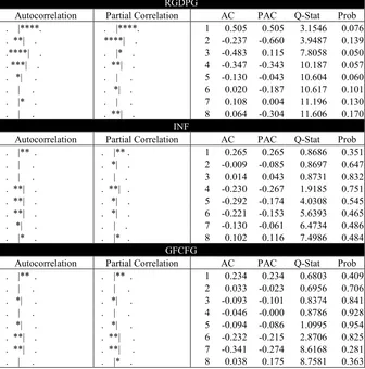
As mentioned in the methodological section, stationarity of the variables are checked by employing the Correlogram test. Test results are given in the Table 2. Based on the test results (mainly according to probability of Q-statistics) one can conclude that all three variables are stationary in the level, i.e. they are I(0). Note that such kind of findings is consistent with result of other studies where growth rates of GDP or CPI or investment demonstrate stationary processes. Note that just for comparison of the results I also applied Unit Root Test by using Augmented Dickey Fuller (ADF) Test (Dickey and Fuller, 1981) for checking stochastic properties of the variables. However, ADF Test results were unreliable as we predicted beforehand.

After making sure that all variables are stationary it may be proceeded with the estimation of equation (1) in order to reveal whether there is any threshold effect of inflation for GDP growth.

3.2 Threshold Model Estimation

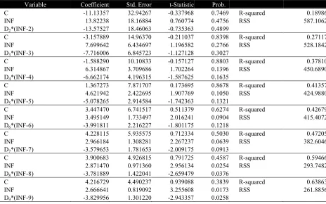
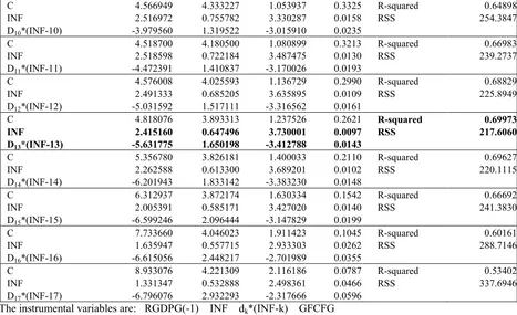
Equation (1) is estimated for each threshold level of inflation, fromk=2tok=17, to minimize RSS or maximize R2. By following Mubarik (2005) and Frimpong and Abayie (2010) firstly Equation (1) is estimated by Least Squares (LS) and then Two-Stages Least Squares is applied in order to prevent possible specification bias of estimations. Note that GFCFG as a control variable becomes insignificant both in LS and TSLS estimations. Therefore, this variable is excluded from specifications, but it is used as instrumental variable in the TSLS estimations.

Results of LS and TSLS estimations are given Table 3 and 4 respectively. According to these tables both LS and TSLS estimation results are very close to each other and indicate that 13 percent threshold level of inflation is satisfactory in terms of minimum RSS and maximum R2. Note that in case of k=13, obtained specifications are economically meaningful and have not any problem with residuals autocorrelation, non-normality, serial correlation, heteroscedasticity and misspecification. In order to save space only results of residual tests as well as misspecification test in TSLS estimation are introduced here, in Table 5 and those in case of LS estimation can be obtained from author under request.

4. Interpretations of Estimation Results

Estimation outputs indicate that threshold level of inflation for GDP growth is 13 percent in Azerbaijani economy. Note that this finding is the same results of Espinoza et al. (2010), 13 percent for oil exporting countries including Azerbaijan and Christoffersen and Doyle (1998), 13 percent for developing countries. It is higher than, 8 percent by Sergii (2009) for transition countries, 11 percent by Khan and Sendhaji (2001) for developing countries while it is lower than 17 percent by Kremer et al. (2009) for non-industrialized countries.

According to Table 3 and 4, inflation which is lower than 13 percent has a positive effect on GDP growth, but this positive relationship becomes negative one when inflation exceeds 13 percent. To be precise, when inflation exceeds the 13 percent threshold, economic growth is expected to decline by about 3 percent



12 2.4151605.631775



.

Thus, monetary decision makers should keep inflation under 13 percent.

It is worth to note that as Kemer et al. (2009) stated, inflation thresholds in developing countries and, thus, the appropriate level of the inflation target might be country-specific. Kemer et al. (2009) recommends that the identification of country-specific inflation thresholds in the inflation-growth nexus might provide useful information about the appropriate location and width of an inflation targeting band.

5. Concluding Remarks and Policy Suggestions

6

Reference

Christoffersen, P. and Doyle, P., (1998), “From Inflation to Growth. Eight Years of Transition”, IMF Working Paper No. WP/98/100

Dickey, D. and W. Fuller, (1981), “Likelihood Ratio Statistics for Autoregressive Time Series with a Unit Root,” Econometrica, Vol. 49

Drukker, D., Gomis-Porqueras, P. and Hernandez-Verme, P., (2005), “Threshold effects in the relationship between inflation and growth: A new panel-data approach”. Proceedings of the 11th International Conference on Panel Data, Feb. 9.http://www.uh.edu/~cmurray/TCE/papers/Drukker.pdf

Espinoza Raphael, Leon Hyginus and Prasad Ananthakrishnan, (2010), “Estimating The Inflation-Growth Nexus-A Smooth Transition Model” IMF Working Paper, WP/10/76

Fabayo, J.A. and Ajilore O.T., (2006), “Inflation-how much is too much for economic growth in Nigeria”. Ind. Econ. Rev., 41: 129-148.http://ideas.repec.org/a/dse/indecr/v41y2006i2p129-147.html

Feldstein, M., (1982), “Inflation tax rules and investment: Some econometric evidence”. Econometrica, 50: 825-62.

http://www.jstor.org/pss/1912766

Frimpong Joseph Magnus and Oteng-Abayie Eric Fosu, (2010), “When is Inflation Harmful? Estimating the Threshold Effect for Ghana” American Journal of Economics and Business Administration 2 (3): 225-232

Gujarati N. Domador, and Porter C. Dawn, (2009), “Basic Econometrics”, The McGraw-Hill, New York, USA

Hussain, M., (2005), “Inflation and Growth: Estimation of Threshold Point for Pakistan”.Pakistan Business Review, October, pp. 1-15

Khan, M. and Senhadji A., (2001), “Threshold effects in the relationship between inflation and growth”. IMF Staff Papers, 48: 1-21.http://ideas.repec.org/a/pal/imfstp/v48y2001i1p1.html

Kremer S., A. Bick and D. Nautz, (2009), “Inflation and Growth: New Evidence From a Dynamic Panel. Threshold Analysis”. SFB 649 Discussion Paper. 2009-036.http://sfb649.wiwi.hu-berlin.de/papers/

Li Min (2006), “Inflation and Economic Growth: Threshold Effects and Transmission Mechanisms” Department of Economics, University of Alberta, 8-14, HM Tory Building, Edmonton, Alberta, Canada, T6G 2H4

Mubarik Ali Yasir, (2005), “Inflation and Growth: An Estimate of the Threshold Level of Inflation in Pakistan” SBP-Research Bulletin. Volume 1, Number 1

Munir Qaiser and Mansur Kasim, (2009), “Non-Linearity between Inflation Rate and GDP Growth in Malaysia” Economics Bulletin, Volume 29, Issue 3

Nasir Iqbal and Nawaz Saima, (2010), “Investment, Inflation and Economic Growth Nexus” Pakistan Institute of Development Economics Islamabad, Pakistan. 21

Ocran, M.K., (2007), “A Modeling of Ghana’s Inflation Experience: 1960-2003”. AERC Research Paper No. 169. African Economic Research Consortium, Nairobi;www.aercafrica.org/documents/rp169.pdf

Sarel, M., (1996), “Nonlinear effects of inflation on economic growth”. IMF Staff Papers, 43: 199-215. http://papers.ssrn.com/sol3/papers.cfm?abstract_id =883204

Sargsyan, G.R., (2005), “Inflation and output in Armenia: The threshold effect revisited”. Preceding of the 3rd International AIPRG conference on Armenia, Jan. 15-16, World Bank, Washington, DC.

http://www.aiprg.net/UserFiles/File/jan-2005/grigorsargsyan.pdf

Sergii Pypko, (2009), “Inflation and economic growth: The non-linear relationship. Evidence from CIS countries” Kyiv School of Economics

Shamim Ahmed and Mortaza Golam, (2005), “Inflation and Economic Growth in Bangladesh: 1981-2005”, Policy Analysis Unit, Research Department, Bangladesh Bank, Working Paper Series: WP 0604

Sidrauski, M., (1967), “Inflation and economic growth”. J. Political Econ., 75: 796-810. http://www.jstor.org/stable/1829572

Stockman, Alan, (1981), “Anticipated Inflation and Capital Stock in A Cash-in-Advance Economy.” Journal of Monetary Economics 8:387–93

[image:8.598.72.346.59.218.2]

Table 1: Descriptive statistics of the variables

RGDPG INF GFCFG

Mean 16.43333 7.788889 22.90069 Median 10.80000 6.700000 18.72194 Maximum 34.50000 20.80000 59.98884 Minimum 9.300000 1.500000 -20.94858 Std. Dev. 9.517747 6.970015 24.62383 Skewness 0.939734 0.829628 -0.044935 Kurtosis 2.238542 2.365484 2.560988 Jarque-Bera 1.542083 1.183402 0.075303 Probability 0.462531 0.553385 0.963049 Sum 147.9000 70.10000 206.1062 Sum Sq. Dev. 724.7000 388.6489 4850.663

[image:8.598.74.410.243.583.2]

Observations 9 9 9

Table 2: The Correlogram test for stationarity of the variables RGDPG

Autocorrelation Partial Correlation AC PAC Q-Stat Prob . |****. . |****. 1 0.505 0.505 3.1546 0.076 . **| . ****| . 2 -0.237 -0.660 3.9487 0.139 .****| . . |* . 3 -0.483 0.115 7.8058 0.050 . ***| . . **| . 4 -0.347 -0.343 10.187 0.057 . *| . . | . 5 -0.130 -0.043 10.604 0.060 . | . . *| . 6 0.020 -0.187 10.617 0.101 . |* . . | . 7 0.108 0.004 11.196 0.130 . | . . **| . 8 0.064 -0.304 11.606 0.170

INF

Autocorrelation Partial Correlation AC PAC Q-Stat Prob . |** . . |** . 1 0.265 0.265 0.8686 0.351 . | . . *| . 2 -0.009 -0.085 0.8697 0.647 . | . . | . 3 0.014 0.043 0.8731 0.832 . **| . . **| . 4 -0.230 -0.267 1.9185 0.751 . **| . . *| . 5 -0.292 -0.174 4.0308 0.545 . **| . . *| . 6 -0.221 -0.153 5.6393 0.465 . *| . . | . 7 -0.130 -0.061 6.4734 0.486 . |* . . |* . 8 0.102 0.116 7.4986 0.484

GFCFG

Autocorrelation Partial Correlation AC PAC Q-Stat Prob . |** . . |** . 1 0.234 0.234 0.6803 0.409 . | . . | . 2 0.033 -0.023 0.6956 0.706 . *| . . *| . 3 -0.093 -0.101 0.8374 0.841 . | . . | . 4 -0.046 -0.000 0.8786 0.928 . *| . . *| . 5 -0.094 -0.086 1.0995 0.954 . **| . . **| . 6 -0.232 -0.215 2.8706 0.825 . **| . . **| . 7 -0.341 -0.274 8.6168 0.281 . | . . |* . 8 0.038 0.175 8.7581 0.363

Table 3: Least Squares Estimation of inflation threshold model from K = 2 to K = 17

Dependent variable: RGDPG

Variable Coefficient Std. Error t-Statistic Prob.

C -11.53355 30.61177 -0.376768 0.7175 R-squared 0.209748 INF 13.79584 16.90395 0.816131 0.4413 RSS 592.9262 D2*(INF-2) -13.51385 17.17413 -0.786872 0.4572

C -2.955567 12.92528 -0.228666 0.8257 R-squared 0.295871 INF 7.635740 5.745780 1.328930 0.2256 RSS 528.3083 D3*(INF-3) -7.652952 6.144866 -1.245422 0.2530

C -1.047769 8.602055 -0.121804 0.9065 R-squared 0.397506 INF 6.176104 3.304335 1.869091 0.1038 RSS 452.0513 D4*(INF-4) -6.522190 3.769633 -1.730193 0.1272

C 1.855880 6.634236 0.279743 0.7878 R-squared 0.431490 INF 4.520316 2.155784 2.096831 0.0742 RSS 426.5533 D5*(INF-5) -4.974919 2.625315 -1.894980 0.0999

[image:8.598.72.536.616.782.2]

8

INF 3.422346 1.538913 2.223873 0.0615 RSS 416.8651 D6*(INF-6) -3.917600 1.999950 -1.958849 0.0910

C 4.671398 4.951818 0.943370 0.3769 R-squared 0.487595 INF 2.899768 1.159076 2.501792 0.0409 RSS 384.4578 D7*(INF-7) -3.511215 1.610957 -2.179584 0.0657

C 4.460734 4.118086 1.083205 0.3146 R-squared 0.604143 INF 2.795725 0.862052 3.243106 0.0142 RSS 297.0114 D8*(INF-8) -3.701707 1.291889 -2.865346 0.0242

C 4.772338 3.756681 1.270360 0.2445 R-squared 0.646367 INF 2.596704 0.727196 3.570844 0.0091 RSS 265.3305 D9*(INF-9) -3.752558 1.185104 -3.166438 0.0158

C 5.089603 3.625721 1.403749 0.2032 R-squared 0.656704 INF 2.453962 0.670788 3.658325 0.0081 RSS 257.5753 D10*(INF-10) -3.904909 1.202851 -3.246378 0.0141

C 5.050061 3.501198 1.442381 0.1924 R-squared 0.676645 INF 2.455188 0.641518 3.827150 0.0065 RSS 242.6129 D11*(INF-11) -4.388942 1.287493 -3.408904 0.0113

C 5.099751 3.374423 1.511295 0.1745 R-squared 0.694506 INF 2.429872 0.609145 3.988987 0.0053 RSS 229.2123 D12*(INF-12) -4.941134 1.386011 -3.565005 0.0092

C 5.306272 3.265148 1.625124 0.1482 R-squared 0.705986 INF 2.359416 0.575826 4.097449 0.0046 RSS 220.5985 D13*(INF-13) -5.539543 1.508855 -3.671356 0.0079

C 5.766795 3.208219 1.797506 0.1153 R-squared 0.703649 INF 2.217782 0.545182 4.067966 0.0048 RSS 222.3521 D14*(INF-14) -6.118578 1.676647 -3.649294 0.0082

C 6.590220 3.245379 2.030647 0.0818 R-squared 0.676792 INF 1.977100 0.519715 3.804202 0.0067 RSS 242.5026 D15*(INF-15) -6.540756 1.918028 -3.410146 0.0113

C 7.827643 3.394162 2.306208 0.0545 R-squared 0.615008 INF 1.627276 0.495288 3.285514 0.0134 RSS 288.8593 D16*(INF-16) -6.595928 2.244050 -2.939296 0.0217

[image:9.598.73.537.492.782.2]

C 8.884087 3.548435 2.503664 0.0408 R-squared 0.549863 INF 1.335484 0.473593 2.819900 0.0258 RSS 337.7378 D17*(INF-17) -6.805829 2.695284 -2.525088 0.0395

Table 4: Two-Stage Least Squares Estimation of inflation threshold model from K = 2 to K = 17

Dependent variable: RGDPG

Variable Coefficient Std. Error t-Statistic Prob.

C -11.13357 32.94267 -0.337968 0.7469 R-squared 0.18986 INF 13.82238 18.16884 0.760774 0.4756 RSS 587.1062 D2*(INF-2) -13.57527 18.46063 -0.735363 0.4899

C -3.157889 14.96370 -0.211037 0.8398 R-squared 0.27117 INF 7.699642 6.434697 1.196582 0.2766 RSS 528.1842 D3*(INF-3) -7.716006 6.845723 -1.127128 0.3027

C -1.588290 10.10833 -0.157127 0.8803 R-squared 0.37810 INF 6.314867 3.709686 1.702264 0.1396 RSS 450.6890 D4*(INF-4) -6.662174 4.196315 -1.587625 0.1635

C 1.367273 7.871707 0.173695 0.8678 R-squared 0.41357 INF 4.621942 2.422695 1.907769 0.1050 RSS 424.9880 D5*(INF-5) -5.078265 2.914584 -1.742363 0.1321

C 3.447470 6.741517 0.511379 0.6274 R-squared 0.42679 INF 3.495149 1.733497 2.016241 0.0904 RSS 415.4072 D6*(INF-6) -3.991811 2.216227 -1.801175 0.1218

C 4.228115 5.935575 0.712334 0.5030 R-squared 0.47205 INF 2.966184 1.308281 2.267237 0.0639 RSS 382.6046 D7*(INF-7) -3.579653 1.781653 -2.009175 0.0913

C 3.900683 4.926815 0.791725 0.4587 R-squared 0.59466 INF 2.871470 0.971360 2.956134 0.0254 RSS 293.7482 D8*(INF-8) -3.781889 1.422041 -2.659479 0.0376

C 4.566949 4.333227 1.053937 0.3325 R-squared 0.64898 INF 2.516972 0.755782 3.330287 0.0158 RSS 254.3847 D10*(INF-10) -3.979560 1.319522 -3.015910 0.0235

C 4.518700 4.180500 1.080899 0.3213 R-squared 0.66983 INF 2.518598 0.722184 3.487475 0.0130 RSS 239.2737 D11*(INF-11) -4.472391 1.410837 -3.170026 0.0193

C 4.576008 4.025593 1.136729 0.2990 R-squared 0.68829 INF 2.491333 0.685205 3.635895 0.0109 RSS 225.8949 D12*(INF-12) -5.031592 1.517111 -3.316562 0.0161

C 4.818076 3.893313 1.237526 0.2621 R-squared 0.69973 INF 2.415160 0.647496 3.730001 0.0097 RSS 217.6060 D13*(INF-13) -5.631775 1.650198 -3.412788 0.0143

C 5.356780 3.826181 1.400033 0.2110 R-squared 0.69627 INF 2.262588 0.613300 3.689201 0.0102 RSS 220.1115 D14*(INF-14) -6.201943 1.833142 -3.383230 0.0148

C 6.312937 3.872174 1.630334 0.1542 R-squared 0.66692 INF 2.005391 0.585171 3.427020 0.0140 RSS 241.3830 D15*(INF-15) -6.599246 2.096444 -3.147829 0.0199

C 7.733660 4.046023 1.911423 0.1045 R-squared 0.60161 INF 1.635947 0.557715 2.933303 0.0262 RSS 288.7146 D16*(INF-16) -6.615056 2.448217 -2.701989 0.0355

C 8.933076 4.221309 2.116186 0.0787 R-squared 0.53402 INF 1.331347 0.532888 2.498361 0.0466 RSS 337.6946 D17*(INF-17) -6.796076 2.932293 -2.317666 0.0596

[image:10.598.72.539.59.344.2]

The instrumental variables are: RGDPG(-1) INF dk*(INF-k) GFCFG

Table 5: Two-Stage Least Square estimation of inflation threshold model at K =13 and test outputs

Dependent Variable: RGDPG Method: Two-Stage Least Squares

Instrument list: RGDPG(-1) C INF D13*(INF-13) GFCFG

Variable Coefficient Std. Error t-Statistic Prob.

C 4.818076 3.893313 1.237526 0.2621

INF 2.415160 0.647496 3.730001 0.0097

D13*(INF-13) -5.631775 1.650198 -3.412788 0.0143 R-squared 0.699730 Mean dependent var 16.43333 Adjusted R-squared 0.599639 S.D. dependent var 9.517747 S.E. of regression 6.022265 Sum squared resid 217.6060 F-statistic 6.990992 Durbin-Watson stat 2.042360 Prob(F-statistic) 0.027073 Second-Stage SSR 217.6060 J-statistic 2.660317 Instrument rank 5.000000

Test Outputs

Residuals Test Autocorrelation Test

Autocorrelation Partial Correlation AC PAC Q-Stat Prob . | . . | . 1 -0.028 -0.028 0.0095 0.922 . *** . . ***| . 2 -0.447 -0.448 2.8360 0.242 . | . . | . 3 -0.011 -0.052 2.8381 0.417 . | . . **| . 4 -0.041 -0.307 2.8714 0.580 . | . . | . 5 0.017 -0.046 2.8788 0.719 . | . . **| . 6 0.010 -0.213 2.8823 0.823 . | . . | . 7 -0.006 -0.057 2.8841 0.896 . | . . *| . 8 0.006 -0.153 2.8874 0.941 Normality Test: Jarque-Bera 0.321909 (0.851331)

LM Test: ARCH Test: White Heteroskedastiklik Testi: F-statistics 0.008297 (0.9274) 0.649023 (0.4512) 3.322954 (0.1358) Obs*R-squared 8.629650 (0.0711) 0.780894 (0.3769) 6.918090 (0.1403)

Misspecification Test Ramsey RESET Testi

t-statistika 0.189540 (0.8571)

F-statistika 0.035925 (0.8571)