Adaptive Back Stepping Control of Automotive Electronic Control Throttle

ISSN Online: 1945-3124 ISSN Print: 1945-3116

Adaptive Back-Stepping Control of Automotive

Electronic Control Throttle

Nobuo Kurihara, Hiroyuki Yamaguchi

Department of System and Information Engineering, Hachinohe Institute of Technology, Hachinohe, Japan

Abstract

Back-stepping control (BSC), which is deemed effective for a non-holonomic system, is applied to improving both responsiveness and resolution perfor-mance of an electronic control throttle (ECT) used in automotive engines. This paper is characterized by the use of a two-step type BSC in a manner that achieves an improvement in responsiveness with the ETC operated in a fully opened state by adding a derivative term in Step 1 and the improvement in resolution performance with the ETC operated in a minutely opened state by adding an adaptive feature in the form of an integral term using the control deviation in Step 2. This paper presents an ECT control expressed as a second-order system including nonlinearities such as backlash of gear train and static friction in sliding area, a BSC system designed based on Lyapunov stability, and a determination method for control parameters. Also, a two-step type BSC system is formulated using Matlab/Simulink with a physics model as a control object. As a result of simulation analyses, it becomes clear that the BSC system can achieve quicker response because the derivative term works effectively and finer resolution because the adaptive control absorbs the error margin of the nonlinear compensation than conventional PID control.

Keywords

Back-Stepping Control, Adaptive Control, Electronic Throttle, Automotive Engine

1. Introduction

The electronic control throttle in automobile engine control systems is indis-pensable to increasing fuel economy and curbing exhaust emissions. It is the main actuator for torque control in gasoline engines and emission control in di-esel engines, and its responsiveness and resolution have to meet strict require-ments. It is anticipated that the electronic control throttle will not only provide a solution to relevant mechanical problems, but also deliver improvements How to cite this paper: Kurihara, N. and

Yamaguchi, H. (2017) Adaptive Back- Stepping Control of Automotive Electronic Control Throttle. Journal of Software En-gineering and Applications, 10, 41-55. http://dx.doi.org/10.4236/jsea.2017.101003

Received: December 16, 2016 Accepted: January 20, 2017 Published: January 23, 2017

Copyright © 2017 by authors and Scientific Research Publishing Inc. This work is licensed under the Creative Commons Attribution International License (CC BY 4.0).

http://creativecommons.org/licenses/by/4.0/

through its method of control.

Research on nonlinear control based on feedback control enhanced by the Lyapunov design method has been in progress since the early 1990’s. Krstić et al. proposed this type of control as “Back-stepping Design” [1], and Zhou et al. then systematized it as “Adaptive Back-stepping Control [2]”. This back-stepping control (BSC) is a promising method applicable to electronic throttle control as a means of solving nonlinear problems, such as the backlash of the gear train and frictional characteristics of rotational sliding. Pan et al. proposed a relevant ap-proach [3], but this focuses on state observers, and does not take advantage of the benefit obtained from BSC. The author et al. has achieved high responsive-ness with the aid of sliding-mode control [4] [5]. However, nonlinear compensa-tion for fine control is insufficient.

This paper describes a method for designing back-stepping control (BSC) of a low-order control object with the nonlinear characteristics expected for an au-tomobile electronic control throttle. The control used is two-step type BSC based on a quadratic linear model so that design can be formulated in a manner simi-lar to that for conventional PID control. We added a derivative control function to Step 1 in order to improve responsiveness, and an adaptive control function to Step 2 in order to absorb model errors in nonlinear compensation. The effects of these functions were examined by simulation using Matlab/Simulink. As con-trol objects, we built a physical model based on the structure of the electronic control throttle, a backlash model for examining the drive torque, and a Stribeck model for consideration of frictional characteristics [6] [7]. The derivative term in Step 1 serves to improve the starting characteristics that the electronic control throttle exhibits in response to sudden acceleration. Minute opening control on the electronic control throttle may cause sticking due to static friction, over-shooting after a motion, and a steady-state deviation due to backlash. The results of simulations suggest that such problems with resolution degradation due to response lag and nonlinear characteristics can be solved by improving Steps 1 and 2 of the two-step type BSC. We also achieved further improvement by refer-ring to a reference linear model.

2. Basic BSC Design

This paper systematizes BSC design by assuming that the control object is an (N ×

N) MISO system that combines the linear and nonlinear characteristics of a state variable. The control object is assumed to be an object described by Equation (1).

( )

( )

( )

1 1, 1

1 , 1 , 1 N j j j N

i i j j i

j

N

N N j j N N

j

x a x

x a x

x a x b u

We designed an N-step control system that feeds back all the components of the state variable. The control law meeting the conditions for Lyapunov stability in each step is given by Equations (2) to (4). Derivation of these equations is omitted.

Step 1:

( )

( 2)

1 1 1 1 1

1 12

1 N j

d j j

j

z c z a x

a

α ≠ ψ

=

 

= _ − − − _



∑

x  (2)

Step i:

( )

( 1)

1 1, 1 ,

1 , 1

1 N j i

i i i i i i i i j j i

j i i

c z a z a x

a

α α− − − ≠ + ψ

= +

 

= _ − − − − _



∑

x  (3)

Step N:

( )

1 1, 1

1

1 N

N N N N N N Nj j N

j N

u c z a z a x

b

α

− − − =

ψ

 

=  − − − − 



∑

x  (4)

where zd is the desired value, and is the control error in Step i.

3. Modeling an Electronic Control Throttle

3.1. Linear Model

[image:3.595.211.541.149.297.2]

Figure 1 illustrates the structure of an electronic control throttle used for auto-mobile engines. Its main elements are a DC motor, gear train (pinion gear, in-termediate gear, and sector gear), butterfly valve, and springs. For these ele-ments, a DC motor circuit equation, DC motor rotational motion equation, gear-train rotational motion equation, and valve rotational motion equation are derived. These physics are shown from Equations (5) to (8).

Table 1 shows the parameter names and their meanings used in the throttle valve’s mathematical models. In addition, Equations (5) to (8) can be reduced to Equations (9) to (10) by considering the gear ratios.

d d

d d

m

m m

i

L Ri K V

t t

θ

[image:3.595.241.532.510.724.2]

+ + = ₍₅₎

[image:4.595.205.542.82.544.2]

Table 1. Parameters of ECT.

Parameters Physical meanings Units

θv Valve opening deg

θm Motor rotary angle deg

V Motor voltage V

Tsp, Tspl Spring torque -

Ng, Nv Gear ratio N∙m

Jm, Jg, Jv Moment of inertia N∙m∙s2

Dm, Dg, Dv Viscous friction N∙m∙s

Eg, Ev Transmission efficiency -

R Motor internal resistance Ω

2 1 2 d d d d m m

m m m

J D K i T

t t

θ

₊

θ

_{= −}

(6) 2 1 2 2 d d d d g g

g g g g

J D N E T T

t t

θ θ

+ = − (7)

( )

2 2 2 d d d d v v

v v v v sp

J D N E T T

t t

θ

₊

θ

_{= −}

_θ

(8)

( )

2 2 d d d d v v sp v

J D T K I

t t

θ

₊

θ

₊

_θ

_{= ⋅}

(9)

d d

m e g v v

i

L Ri K N N V

t+ + ⋅ ⋅ ⋅θ = (10) where

2 2 2

2 2 2

m g v g v g v v v

m g v g v g v v v

m g g v v

J J N N E E J N E J

D D N N E E D N E D

K K N E N E

= ⋅ ⋅ ⋅ ⋅ + ⋅ ⋅ +

= ⋅ ⋅ ⋅ ⋅ + ⋅ ⋅ +

= ⋅ ⋅ ⋅ ⋅

3.2. Nonlinear Model

We consider the backlash characteristics described by Figure 2 and Equation (11) and the friction characteristics described by Figure 3 and Equation (12) as the nonlinear characteristics of the electronic control throttle. The friction cha-racteristics are known as the Stribeck model and are obtained as a composite of static, Coulomb, and viscous friction. Since the viscous friction is already con-tained as the Dθv term of Equation (9), it is excluded when Tst

( )

θv expressed by Equation (12) is applied.

( )

( )

( )

( )

(

( )

)

( )

( )

(

( )

)

if 0 and

or if 0 and

0 otherwise

v v v v r

v v v v l

mT t T t T t m T t B

T t T t T t m T t B

 ≥ = −



=_ < = −

 

 

[image:5.595.259.488.69.220.2]

Figure 2. Backlash characteristics of gear train.

Figure 3. Stribeck friction nonlinearity.

( )

(

(

)

(

)

)

( )

(

)

(

)

(

)

(

)

if

exp

if

exp v th

c brk c s v v v v

st v

v th

c brk c s v v v v th

T T T c sign D

T

T T T c D

θ θ

θ θ θ

θ

θ θ

θ θ θ θ

 _≥



 _{+ − − +}

 = 

<  

 _{+ − − +}



 

  



 

   

(12)

3.3. Electronic Control Throttle

The block diagram in Figure 4 is obtained by combining the linear model in 3.1 and nonlinear model in 3.2. As the physical model of an electronic control throt-tle, it is used as a control object in the creation of a control model or for con-firming the performance of a control system.

3.4. Linear Control Model

[image:5.595.270.472.255.447.2]

qua-dratic linear model in order to ensure consistency with conventional PID control systems. Assuming a control model expressed by Equation (13), we identified the step response of the electronic control model of Figure 4 with the nonlinear model excluded. We thereby obtained a second-order delay model that is in good agreement with the physical model, as can be seen in Figure 5.

1 2

2 21 1 22 2 2

x x

x a x a x b u

= 

 = + +

 

[image:6.595.60.540.154.463.2]

 (13)

Figure 4. Block diagram of electronic control throttle.

Time [s]

[image:6.595.135.462.460.711.2]

4. Detailed Design of BSC

When designing the BSC control system for the electronic control throttle, we changed the control object from Equation (1) to Equation (13) by reducing its order. This control object is a quadratic linear model suited to the control model derived in the preceding section with a friction and backlash model added. In the Equation (14), x1 is the throttle opening, ψ2

( )

x2 the friction torque, and

( )

B  the backlash function.

( )

( )

1 2

2

2 2 2

1 i i i

x x

x a x x bu

u B v

ψ =  =   = + +    = 

∑



 (14)

The BSC is a two-step type of control consisting of Step 1 for the x1 feedback and Step 2 for the x2 loop.

4.1. Adding a Derivative Term to Step 1

In this study, we added a derivative term to Step 1 in order to improve respon-siveness (particularly the starting characteristics). The following demonstration of stability omits description of nonlinear characteristics.

Equation (15) defines the control law of Step 1 using a linear combination of a control deviation z1 and its change rate z1.

(

) (

)

1 zd c z1 1 d z1 1 c1 0 d1 0

α = − +  > ≥ (15) For the Lyapunov candidate function V1 defined by Equation (15), we ob-tain:

2

1 1

1 2

V = z (16)

1 1 d

z = −x z (17)

1 1 d 2 d

z = −x z =x −z (18)

(

)

(

)

(

)

(

)

1 1 1 1 2

1 2 1 1 1 1 1

2

1 1 1 1 1 1 2 1

2

1 1 1 1 1 2

2 1 1 1 2 1

1 1

d

V z z z x z

z x c z d z

c z d z z z x

c z d V z z

c z z z

d α α = = − = − − − = − − + − = − − + = − + +  _{ }    (19)

With Step 2 designed such that the intermediate control deviation z2 =0, the following inequality holds.

1 0

(

)

2

2 1 2

1

1 2 1

V V z

d

= +

+ (21)

By differentiating both sides, we obtain the following.

(

2 2

) (

)

(

2 2

)

2 1 1 1 2 2

1 1

1

0

1 1

z z

V V c z c z

d d

= + = − − ≤

+ +



  ₍₂₂₎

Since V2 is a Lyapunov function, this inequality shows that Step 2 is stable, with the intermediate control deviation z2 converging to zero.

Equation (22) is derived as follows.

(

)

(

1

)

2

2 1 1 2 2 1 1 2 2 2 2 2 1

1

1 1

V c z z z z a x z a x z bu z

d α

= − + + + + −

+

 _{ (23)}

Assuming that the control law u is given by Equation (24), Equation (25) is obtained by substituting Equation (24) into Equation (21).

(

1 2 2 1 1 2 2 1

) (

2

)

1

0

u c z a x a x z c

b α

=  − − − − > (24)

(

)

(

)

(

)

(

)

1

1 2

2

2 1 1 2 2 1 1 2 2 2 2 1 2 2 2 1 1 1 2 2 1

1 2 2 1 2 1 1 1 1 1 0 1

V c z z z z a x z a x z z b c z z a x a x

d b

c z c z d α α    = _− + + + − + _ − − − − + _ +    = − − ≤ +  _{ } (25)

A stable control system can therefore be achieved by using Equation (24) as the control law for the BSC.

4.2. Adding an Integral Term to Step 2

Headings, or heads, are organizational devices that guide the reader through your paper. There are two types: Component heads and text heads.

As shown by Equations (2) and (3), BSC has the advantage of allowing nonli-near compensation to be easily achieved. When the friction function ψ2

( )

x2 is known, Equation (25) can be used as the control law for Step 2.

(

1 2 2 1 1 2 2 2 1

) (

2

)

1

0

u c z a x a x z c

b α ψ

=  − − − − − > (26)

In actual applications, however, nonlinear characteristics contain errors or are unknown. In addition, the backlash function B

( )

 and other characteristics need to be offset not by subtraction but with an inverse model. In this study, those issues were solved by adding an adaptive control term fad

( )

z2 that inte-grates the control deviation z2 in Step 2 under the conditions for Lyapunov stability. Equation (26) or (27) can be applied as the adaptive control term

( )

2 ad

f z .

( )

(

*

)

2 2 2 2 d

ad

f z z ⋅

∫

ς

z −z t (27)

( )

( )

(

*

)

2 2 2 2 d

ad

f z sign z ⋅

∫

η

z −z t (28)

In these equations, * 2

deviation. If an adaptive control term is added, the control law is given by Equa-tion (29).

2

*

2 2 1 2 1

1

1

i i ad

i

u a x c z z f

b = ψ α

 

= _− − − − + − _



∑

  (29)

In this case, since Equation (27) can be expressed as Equation (30), stable control is guaranteed.

(

)

(

1 2

)

2 2

2 1 2 2

1

1

0

1 ad

V c z c z z f

d

= − − − ≤

+

 ₍₃₀₎

4.3. Adaptive BSC System

Figure 6 shows a block diagram of the adaptive back-stepping control system obtained from the above design. The backlash function is disregarded based on the following results of paragraph 5.3. The reference linear model in Figure 6 is the BSC system assumed without nonlinear control model and without parame-ter error margin of linear model and is not indispensable.

5. Simulations and Discussion

5.1. Improvement in Response

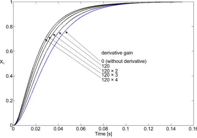
[image:9.595.64.541.446.720.2]

We examined the control performance of the BSC system by measuring the step response. Assuming that the control object has the physical characteristics shown in Figure 4, we used Matlab/Simulink and built the BSC system illu-strated in Figure 6. The derivative term added to Step 1 improved the starting characteristics but delayed convergence near the desired value. To solve this

problem, we attached an imperfect dead zone expressed by Equation (31) to the subsequent stage of the derivative term (also included in Figure 6). This dead zone makes the control deviation z1 minute and gradually reduces the deriva-tive term gain. The Step 2 parameters a a b1, 2, were determined by fitting the control object to Equation (11).

( )

( )

(

( )

)

e z ti L 1

o i

z t =z t +L − − (31)

Figure 7 shows the results of the simulation. Response becomes higher with increasing derivative term gain in Step 1. This effect gradually becomes smaller, and the response does not exceed critical damping, so that no oscillation is ob-served.

5.2. Setting Control Parameters

The control parameters to be adjusted in designing the BSC are, in Step 1, the proportional term gain c1 of the control deviation z1 and the derivative term gain d1, and, in Step 2, the proportional term gain c2 of the intermediate con-trol deviation z2 and the parameters a a b1, 2, of the linear control model ex-pressed in Equation (13). The parameters a a b1, 2, can be adjusted by fitting them to the step response of the control object. The proportional term gains c1 and c2, which are unique to the BSC, are mutually complementary, as shown in Table 2 which lists the simulation results. Hence, c c1 2 is determined by consi-dering factors such as the constraint on the operation quantity u t

( )

, and

( )

[image:10.595.213.536.492.718.2]

supu t , the constraint on the controlled quantity x1, and avoidance of over-shoot. Next, c c1 2 is determined from the response speed of the controlled quantity x1, for example, a 95% response in 80 ms. The remaining derivative term gain d1 in Step 1 is determined by varying it from d1=0 such that the target responsiveness is ensured under the above-mentioned constraints.

5.3. Compensating for Backlash Characteristics

Backlash is included as Equation (11) in the control object. As shown in Equa-tion (14), the relaEqua-tionship between the input u and output v of the control model is expressed as u=B v

( )

. This suggests that backlash compensation re-quires an inverse model. In this study, we assumed that the backlash was un-known and examined how effectively the adaptive control term fad

( )

z2 ab-sorbed it in Step 2. We implemented the simulation using Equation (32), which was obtained by omitting *

2

z from Equation (27).

( )

2 2 2 d

ad

f z z ⋅

∫

ς

⋅z t (32)

Figure 8 shows the simulation results. As the backlash motion is repeated, the effect of the adaptive control term causes the motion to gradually approach that without backlash (zd). The results show that this tendency also differs depending on the BSC control parameter c1 × c2. It can be seen that, when c1 × c2 is sufficiently large relative to the width of the backlash dead zone, good respon-siveness is obtained even without the adaptive control term.

5.4. Compensating for Friction Characteristics

[image:11.595.208.538.402.714.2]

Since the electronic control throttle needs to perform fine air-intake adjustment, the responsiveness to be achieved when the target degree of opening is changed

Table 2. Adjustment of control parameters.

Case c1 c2 c1/c2 c1c2 Re s. at 80 ms

○_{1 60 60 1.00 3600 95}

○_{2 45 80 0.56 3600 94}

○_{3 36 100 0.44 3600 93}

○_{4 30 120 0.36 3600 91}

○_{5 40 90 0.25 3600 88}

on a continuous basis by 0.05˚ intervals is given as the target specification. In the operation of such minute openings (NOT: Narrow Open Throttle), friction cha-racteristics have a relatively large influence. In this simulation, we used the fric-tion compensafric-tion model *

( )

2 x2

ψ

_{expressed by Equation (33).}

( )

( )

*

2 x2 2 x2

ψ

= ⋅

ξ ψ

₍₃₃₎ The friction characteristics are known when ξ=1, contain an error when 1> >ξ 0, and are unknown when ξ =0.

The simulation was implemented with a step response of 0.025˚, and includes the effect of adding the adaptive control term fad

( )

z2 . The results are given in Figure 9 and Figure 10.

Figure 9 shows the results corresponding to ξ =0.7. It can be seen that the

throttle does not operate without compensation for the static friction being ap-plied. In addition, a large control deviation remains when compensation is im-plemented using only the friction compensation model *

( )

2 x2

ψ

. In contrast, the response is in close agreement with that corresponding to the no-friction state when the adaptive control term fad

( )

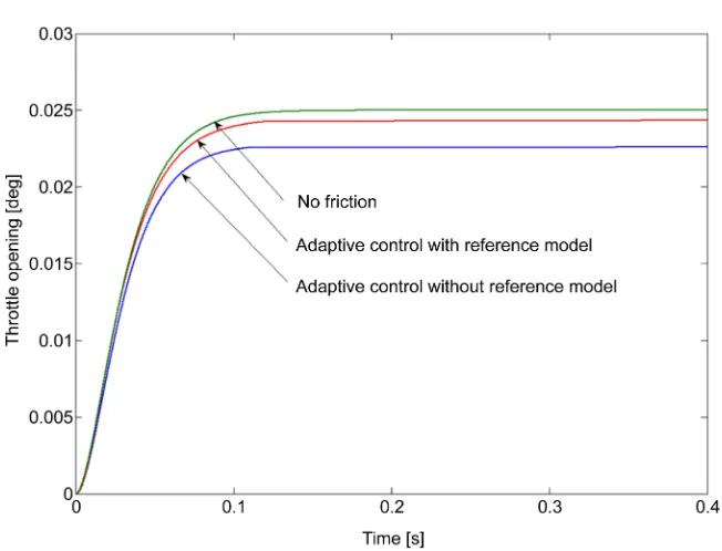
z2 is added.

Figure 10 shows the results for ξ = 0, in which no friction compensation model is used since the friction characteristics are unknown. Although a steady devia-tion remains when only the adaptive control term fad

( )

z2 is added, it can be reduced using the control deviation z2 of Step 2 of the reference linear model.

5.5. Evaluating Electronic Throttle Control

Figure 11 shows the results of simulating operation of the electronic control throttle from the fully closed to fully open position (WOT: Wide Open Throt-tle), and compares it with operation using conventional PID control. All of the

Time [s]

[image:12.595.211.536.472.716.2]

[image:13.595.210.536.60.309.2] [image:13.595.211.539.343.574.2]

Figure 10. Responses when friction function is unknown (ξ =0).

Figure 11. Test of Wide-Open-Throttle.

operations meet the 95% response in 80 ms required as the target specification. It can be seen that the starting characteristics are improved by adding a deriva-tive term to Step 1 (D-BSC). Responsiveness can be adjusted by PID control, but too large a derivative term gain will cause overshooting. Critical damping is not exceeded with BSC.

[image:14.595.212.538.69.322.2]

Figure 12. Test of Narrow-Open-Throttle.

and friction characteristics, making it indefinite. However, a resolution of 0.05˚ is required as the target specification of the equipment. In contrast, the effect of the compensation expressed by Equation (26) of Step 2 allows BSC to keep up with minute changes in the desired value.

6. Summary

Back-stepping control (BSC) can compensate separately for linear and nonlinear characteristics in the system design, and provide a stable response even when model errors are present. This study applied BSC to an electronic control throt-tle for automobiles, and thereby achieved improvements in both responsiveness and resolution performance. We expressed a general-purpose design method for BSC as Equations (1) to (4), and determined the following through the use of simulations.

(1) Two-step type BSC is suitable for electronic control throttles.

(2) We presented Equation (13) as the control law for a derivative term added to Step 1 of the two-step type BSC. This improves starting characteristics.

(3) We presented Equations (23) and (24) as control laws for an integral term added to Step 2 of the two-step type BSC (adaptive BSC). This absorbs errors that occur in nonlinear control models.

(4) Consideration of backlash compensation becomes unnecessary if the con-trol gain (c1×c2) of the BSC is increased.

(5) Adaptive BSC allows the desired value to be followed even when friction characteristics are unclear (ξ=0.7) or unknown (ξ =0).

and resolution performance than conventional PID control.

Acknowledgements

We will express our gratitude for Hiroshi Hayashi, Masahiro Miura, and Hiroki Toda that advances the simulation examination in this research.

References

[1] Krstić, M., Kanellakopoulos, I. and Kokotović, P. (1995) Nonlinear and Adaptive Control Design. Wiley-Interscience, New York.

[2] Zhou, J. and Wen, C.Y. (2008) Adaptive Backstepping Control of Uncertain Sys-tems. Springer Publication, Heidelberg.

[3] Pan, Y.D., Ozguner, U. and Dagci, O.H. (2008) Variable-Structure Control of Elec-tronic Trottle Valve. IEEE Transactions on Industrial ElecElec-tronics, 55, 3899-3907.

https://doi.org/10.1109/TIE.2008.2005931

[4] Zhang, Y. and Kurihara, N. (2011) An Integral Variable Structure Compensation Method for Electronic Throttle Control with Input Constraint. Proceedings of 2011 3rd International Conference on advanced Computer Control (ICACC), 18-20 Jan-uary 2011, 492-496. https://doi.org/10.1109/ICACC.2011.6016461

[5] Zhang, Y. and Kurihara, N. (2012) A Study of Integral Sliding Mode Control with Input Constraint for Engine Idling-Speed Control. IEEJ Transactions on Electrical and Electronic Engineering, 7, 214-219.

[6] Brian, A.-H., Dupont, P. and De Wit, C.C. (1994) A Survey of Models, Analysis Tools and Compensation Methods for the Control of Machines with Friction. Au-tomatica, 30, 1083-1138. https://doi.org/10.1016/0005-1098(94)90209-7

[7] Iwasaki, M., Kitoh, Y. and Matsui, N. (1996) Analysis and Performance Improve-ment of Motor Speed Control System with Nonlinear Friction. IEEJ Transactions on Electronics, Information and Systems, 116, 96-102.

Submit or recommend next manuscript to SCIRP and we will provide best service for you:

Accepting pre-submission inquiries through Email, Facebook, LinkedIn, Twitter, etc. A wide selection of journals (inclusive of 9 subjects, more than 200 journals)

Providing 24-hour high-quality service User-friendly online submission system Fair and swift peer-review system

Efficient typesetting and proofreading procedure

Display of the result of downloads and visits, as well as the number of cited articles Maximum dissemination of your research work

Submit your manuscript at: http://papersubmission.scirp.org/