The Detection and Empirical Study of Variance Change Points on Housing Prices —Taking Wuhan City Commodity Prices as an Example

http://www.scirp.org/journal/jmf ISSN Online: 2162-2442

ISSN Print: 2162-2434

The Detection and Empirical Study of Variance

Change Points on Housing Prices

—Taking Wuhan City Commodity Prices as an Example

Huihui Shen

1,2

1_{China University of Geosciences, Wuhan, China}

2_{Department of Statistics, Hubei University of Economics, Wuhan, China}

Abstract

Economic system mathematical model often contains multiple variance change points about structure model. In the same mean, we combine the Bayesian method with the maximum likelihood method on the detection of the variance multiple change points. With Bayesian method, we can eliminate extra parameters first, and then use maximum likelihood method to find the change position. So we both can eliminate extra parameters and can avoid the change point on the prior distribution unknown problem. In addition, the benefit of the maximum likelihood method is just needed to find out likelihood density function of the maximal solution in the solution space, thus the variance of multiple change point detection problem is re-solved. By making substantial analysis with an example from commodity house pric-es in Wuhan, three changpric-es of variance are found in all. They corrpric-espond to the ma-jor structure changes of contemporary property market in Wuhan city. The method is practical and effective as the final results shown. It also has a certain practical sig-nificance.

Keywords

Change Point, Bayesian Method, Maximum Likelihood Method, Commodity House Prices, Joint Distribution Density Function

1. Introduction

With the rapid economic development of modern society, we need to deal with more and more economic and financial problems. Economic cycle of change point analysis

has always been a problem concerned by economists and statisticians [1]. The change

How to cite this paper: Shen, H.H. (2016) The Detection and Empirical Study of Va-riance Change Points on Housing Prices. Journal of Mathematical Finance, 6, 699- 710.

http://dx.doi.org/10.4236/jmf.2016.65049 Received: August 10, 2016*

Accepted: November 7, 2016 Published: November 10, 2016

Copyright © 2016 by author and Scientific Research Publishing Inc. This work is licensed under the Creative Commons Attribution International License (CC BY 4.0).

http://creativecommons.org/licenses/by/4.0/

point identification has played a vital role in the economy. Because the problems about change point greatly help to adjust economic policy and develop long-term and stable

economic in the economic cycle [2]. The realty business is an important pillar industry.

Commercial housing consumption pulls our country’s economic development, but many problems appear in the process of the sharp development of the realty business. So by the analysis and research on the commercial housing price, we find the factors affecting housing prices, and grasp the contradiction of the housing industry in Wuhan city. We try to find the crux of the problem from the price mechanism, the structure of housing supply, housing market price system and the macroeconomic regulation and control, etc., which provides suggestions for the government to perform effective ma-croeconomic regulation and management in the realty business. At the same time they provide a reference on market decision for realty business enterprises and personal in-vestment.

Generally, there are many ways to estimate change point, such as Schwarz informa-tion criterion method, Binary segmentainforma-tion method, Bayesian method, maximum like-lihood method, the likelike-lihood ratio test, (weighted) Least square method, nonparame-tric method, cumulative sum method, etc. Schwarz information criterion is set up in

1978 by Schwarz [3]. The reference [4] is used to detect the existence of the transition

point, and doesn’t need to export its complex distribution function, so the use of in-formation criterion to estimate the number and position of changing point is relatively simple. Binary segmentation method proposed by Vostrikova (1981) can simulta-neously detect the transition point number and their position, and can save a lot of

computation time [5]. In literature [2] the author combined with the previous methods,

which was a combination of Binary segmentation method and Schwarz information criterion method, to detect the mean change points.

A likelihood-ratio method to detect changes in gamma distribution parameter for

general values of the scale parameter was adapted in the reference [6]. The reference [7]

considers the detection problem of variance change point in linear process with long memory. They propose the ratio test to detect the variance change point. The limiting

distribution for test statistics under H0 is derived and the consistency of the test is also

established. The reference [8] uses the cumulative sum of squares method to tackle the

multiple variance change-points issue, in a way similar to the Binary Segmentation ap-proach, this method only needs a small amount of calculation, but detecting change points must use the entire time series segmentation, which is difficult to guarantee the

change point being the global significance. The references [9][10][11] and [12] use the

Bayesian method to detect change point problems.

The reference [13] uses the method of maximum likelihood estimation to estimate

distribution parameters’ change point problem for a series of random variable with in-dependent identically exponential distribution, but the method is an approximate result

in search of transition point location. The reference [14] today proposes a new method

Through the reference [14], I am learning the neural network, and my next work will use deep learning method to detect change point model.

However, the parameters will change with time; in the reference [13] it used

maxi-mum likelihood method to estimate parameters on change point. For general change point problems, we usually consider the changes on the mean and variance, and under the framework of hypothesis test the population distribution is normal in the model, so change point problem of inference is equivalent to the mean or variance change

detec-tion [15].

2. The Variance Change Point Detection

Change point definition: according to the statistical definition, to a certain random va-riable sequences, if there is a point in time, the sequence before the point to a kind of probability distribution and after this point in time sequence to another kind of proba-bility distribution (or the same kind of probaproba-bility distribution but parameters of dif-ferent), so there is a change point in the sequence. The problem of a change point con-tains two aspects as follows: 1) to confirm whether there is any change, 2) to estimate the number and position of unknown change-point.

The typical objective of a change point analysis is to identify how many change points a series has and where they occur.

The reference [10] proposes to use a Bayesian approach to study the mean and

va-riance change point model for the cases of one change and propose to use a sliding window to search for all copy number variations on a given chromosome. the reference

[16] combine the X control chart with the Bayesian estimation technique. Bayesian

estimator with the informative prior is more accurate and more precise when the means of the process before and after the change point time are not too closed. Paul J. Plummer and Jie Chen (2014) examine the problem of locating changes in the distribu-tion of a Compound Poisson Process where the variables being summed are indepen-dent iindepen-dentically distributed normal and the number of variable follows the Poisson

dis-tribution [17]. A Bayesian approach is developed to identify the location of significant

changes in any of the parameters of the distribution, and a sliding window algorithm is used to identify multiple change points.

Pignatiello and Samuel (2001) used the EWMA and cusum charts and the maximum

likelihood estimator (MLE) to estimate the change point of a process [18]. The

refer-ence [19] derived the change point estimators under the case where the S chart and

MLE are used in a gamma process. Later, the reference [20] is that the maximum

like-lihood estimator of a multivariate Poisson process change point is derived for unknown changes that are assumed to belong to a family of monotonic changes.

Consider

{ }

xt , t=1, 2,,T , a series of independent observations from a normal

distribution with mean 0 and variance 2

t

σ

,

(

2

)

~ 0,

t t

x N

σ

, where

2

0 1

2

1 1 2

2 2

2 2 3

2 if 1 if if if t m m t k k t k k t k

k t T τ τ σ τ τ  ≤ ≤  < ≤  

=_ < ≤ 



 _{< ≤}





where 1≤k1<k2<k3<<km<T denote the indexes of the observations before the

variance changes and m is the number of variance changes. There are dj=kj+1−kj

observations with error variance 2

j

τ _,

j

=

0,1,



,

m

. Convenient for expressing and

0 0, m1

k = k + =T . Change points subscript k=

(

k k1, 2,,km

)

′, change points time series

is divided into m+1 period of time, every time distribution xt of is the same:

( )

2

~ 0,

t j

x N τ , k_j < ≤t k_j+₁, j=0,1,,m, m=1, 2,,T−1.

The main question now is how to estimate the location k=

(

k k1, 2,,km

)

′ and the

numbers of the change point according to the sample of x=

(

x x1, 2,,xT

)

′.

We detect variance change point,

(

) ( )

2

d

DX =

∫

_−∞+∞ x−EX f x x it can be seen that

the variance is sample distribution density function, so the detection and analysis of the variance change point ultimately is considered to be the sample density function esti-mation, and then we use the maximum likelihood method to estimate the location of the change point.

(

2

)

~ 0, , 1, 2, , ,

t t

x N σ t=  T then the joint distribution density function of the

ob-servations x=

(

x x1, 2,,xT

)

′, as well as the likelihood function is:

(

1, 2, , n;

)

(

1;

) (

2;

)

(

n;

)

(

; , ,

)

(

| , ,

)

L x x  x

σ

= f x

σ

f x

σ

f x

σ

=L x

σ

k m = f x

σ

k m

(

)

(

)

( )

( )

(

)

2 2 2

1 2

2 2 2

1 2 2 2 2 2 1 2 2 2 2 1 1

2 2 2

1 2 1 2 2 T 1 1 2 1 1 1 2 2 1 2 1 2

1 1 1

; , , | , , e e e

2π 2π 2π

1 1 1

e e 2π _2π 1 1 e e 2π 2π T T T t t t t t T T t t

t t t t

x x x

T x x T _T t t T

x T x

T T

T

L x k m f x k m σ σ σ

σ σ

σ σ

σ σ

σ σ σ

σ _{σ σ σ}

σ σ σ

σ σ σ

= = = − − −   −  − _{ }   = − − − ∑ ∑ ∑ = = × × ×   =_{ } ⋅ =     = _{=  }  

∏

   

where σ =

(

σ σ1, 2,,σ ′T

)

, k

(

k k1, 2, ,km

)

′

=  , and m is the number of the change-

points.

In terms of the reference [11], it gives the joint distribution density function as

fol-lows:

(

)

(

)

1 2 2 1 1 2 0 1 1

| , , e ; , ,

2π k j t t k j j j

T _m x

d

j _j

f x τ k m τ L xτ k m

τ + = + − = ∑   =_{ } ⋅ =

 

Π

(1)

points, and 2 2

j t

τ =σ _, d_j=k_j+₁−k_j ,

(

t=1, 2,, ;T j=0,1,,m

)

, kj < ≤t kj+1 ,

0 0

k = , km+1=T.

3. Bayesian Approach to the Change-Point Problem

We want to solve the key parameter k and m, that is the change point location and the

numbers of change points, and

τ

_{relatively unimportant, is considered to be a}

redun-dant parameter. If we directly use the maximum likelihood method to deal with the re-dundant parameter, there are a lot of difficulties because of the unknown information of

σ

and

τ

. However, the Bayesian method can deal with this problem. The posterior

distribution density function of the parameters can be obtained by using the Bayesian

formula. And then can get the marginal distribution density function of k and m

through the integration of the posterior distribution density function of

τ

_.

To apply Bayesian method expunction extra parameters, we must construct the prior

distribution of

τ

_{. In the absence of good prior information of}

τ

_{, empirical Bayesian}

method can solve the problem. Empirical Bayesian’s thought is to construct the prior

distribution of

τ

_{from the sample information.}

With the above information,

(

2

)

~ 0,

t t

x N

σ

, 2 2

j t

τ =σ _, k_j < ≤t k_j+₁, dj =kj+1−kj,

Under the condition of given k and m are as follows:

( )

1 2 2 2 1 ~ j j k t j t k j

x

d

χ

τ

+

= +

∑

(2)

Thus we can derive the distribution of τj according to the type (2), and use it as the

prior distribution of τj. And then we get the prior distribution of

τ

. The prior

dis-tribution of

τ

_{contains the sample information, so we use the Bayesian method.}

Combining with the type (1):

For 1

( )

2 2 2 1 ~ j j k t j j

t k j

x

y

χ

d

τ

+

= +

=

∑

_, y=

₍

y y₀, ₁,,ym

₎

′,

j

=

0,1,



,

m

, then

1 1 2 2 1 1 j j k j t t k j x y τ + = +   = _ _ 

∑

 ,

( )

1 2 2 2 1 e 2 2 j j j d y

j d j

j

f y y

d

− −

=

  Γ    

(

yj>0

)

(

, | ,

)

(

| , ,

) (

| ,

)

f x

τ

k m = f x

τ

k m f

τ

k m , on both sides of the equation at the same time

integration for

τ

(

)

(

)

(

) (

)

(

)

| ,

, | , d | ,

| , , | , d

| , , k m

f x k m f x k m

f x k m f k m Eτ f x k m

τ

τ

τ

τ

τ

τ

= = = _ _

∫

∫

4. MLE of the Change Point

By type (1):

(

)

1 2 2 1 1 2 0 1 1

| , , e

2π k j t t k j j j

T _m x

d

j _j

f x

τ

k m τ

τ

+ = + − = ∑   =_{ } ⋅

The likelihood function is as follows:

(

)

(

)

(

)

(

)

( )

1

1 ₂ 2 1 1 1 2 2 1 0 1 1 2 2 2 0 0 ₂ 2 1 0 ; , | , | , , 1

| , , d

1 1 1

e e d

2π 2 2 1 1 2π j j k j j j t t k j j j j j j y k

j j j t

t k j

T _m x d y

j j

d d

j _{j j}

T _m k

t t k

j j

L x k m f x k m E f x k m

f x k m f y y x y y y d x y τ τ τ τ τ + + = + + +∞ = + − +∞ _{− −} = = + = ∑ = = _ _       = _ = _ _{ }         = _{ } ⋅ × ⋅ ⋅     Γ      =    

∑

∫

∏

∫

∑

∏

1 1 2 ₁

2 2 2

0 ₂

2

1

2 _{2 2 2 2}

1

0 0 ₂

2 2 1 0 2 1

e e d

2 2

1 1

e e d

2π 2 2 1 1 2π 2 2 j

j j j

j

j

j j j j

j j j j j j j d

y d y

j j

d j

d

T m k d y d y

t j d j j

t k

j j

d

T _m k

t d

t k

j _j

y y

d

x y y y

d x d + + − +∞ _{− − −} − +∞ _{− − −} = + = − = + =   ⋅ ⋅ ⋅     _{ }

  _{Γ }

      =_{ } _ _ ⋅ ⋅ ⋅     _{ } Γ        =_{ } _ _ ⋅     _{ } Γ  

∫

∑

∏

∫

∑

∏

( )

1 1 1 1 0 2 1 2 1 0 0 2 2 2 ₂ 1 0 2 2 1 0 e d

1 1 1

e d 2π 2 2 1 2 2π 2 1 2 2π j j j j j j j j j j j j j j j d y j j d

T m k

d y

t d j j

t k

j j

d

T m k d

j t

t k

j j

T _m d k

t t k j

y y

x y y

d d x d x + + + +∞ − − − _+∞ − − = + = − − = + = − = + = ⋅ ⋅      =_{ } _ _ ⋅ ⋅ ⋅     _{ } Γ    Γ     =_{ } _ _ ⋅ ⋅     _{ } Γ       =_{ } ⋅_   _

∫

∑

∏

∫

∑

∏

∑

∏

( )

( )

( )

1 0 1

1 2 2 2 2 1 0 2 2 2 1 0 2 1 2 2π 2 1 2 2π 2 j j m j j j j j d j j d

T _m k k k

j t

t k

j j

d

T T m k

j t t k j j d d d x d d x d + + + − − − − = + = − − = + = Γ  ⋅  _{ }

 _{Γ }

  Γ     =_{ } ⋅_ _ ⋅     _{ } Γ    Γ     =_{ } ⋅ _ _ ⋅     _{ } Γ   

∑

∏

∑

∏

(

( )

1

0

e d j j

d y

j j j

d y y

+∞

− −

Therefore, we want to use the Bayesian method, also need to know the prior

distribu-tion of m. The prior information of m is unknown, which plays a crucial role in solving

problem. We use the maximum likelihood method to calculate k and m according to

the above joint density function that is the likelihood function. Thus we can avoid the

problems of the prior distribution information of m unknown. We first give m with an

initial value, and then we determine k mˆ | as the location estimation of the change

point number is m by the maximum density function.

5. Empirical Analysis

Housing price problem is the core of the realty business market, housing price is related to the people to live and work in peace and contentment in China, relates to the healthy

development of the real estate market [21]. In the process of the whole real estate

mar-ket, the price mechanism is always a basic adjustment mechanism, the rationality of the price or not also affects the realization of the real estate policy goals, to restore the real estate market in the current country commodity housing boom continuous research of the new policy environment, the deputy provincial city housing prices in Wuhan em-pirical research has practical significance.

The commodity house prices in Wuhan from 2000 to 2015 are as shown in Table 1.

[image:7.595.192.552.402.700.2]

Since the housing system reform in 1998, the Wuhan city real estate development in-vestment into a new historical period, and quickly formed a new real estate boom, the

Table 1. Commercial housing sales price (Yuan/square meters) from 2000 to 2015 in Wuhan city.

Year Average sale price

2000 1983.52

2001 2065.32

2002 2327.21

2003 2353.4

2004 2667.64

2005 3345.75

2006 3622.20

2007 4685.32

2008 4883.01

2009 5265.91

2010 6184.49

2011 6414.72

2012 6349.74

2013 7213.70

2014 8179.25

rising trend of real estate industry has lasted for 15 years. With a nationwide real estate boom climate, statistics show that: 16 years in Wuhan commodity house average price rose from 1983.52 Yuan/square meters to 8861.00 Yuan/square meters, the average an-nual growth of 13.14%.

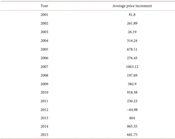
As is shown in Table 2, the average increment of house prices in every year is got by

the data in Table 1.

From the annual sales average increment data shows upward trend since 2001, the price fell slightly after 2012, down 1.01%, but the price increases for three consecutive years since 2013.

In the process of trying to find a place to change point, we first give m with an initial

value, for m = 1, and then maximizing p x k m

(

| , =1

)

can be calculated to k mˆ | =1.

Using change point solution of consistency, we put the m components of k mˆ | as the

estimations for solution of the m components of k mˆ | +1, and maximizing p x k m

(

| ,

)

can be got the estimation of another component. According to the nature of the optim-al solution which each component of the optimoptim-al solution must be mutuoptim-ally

condition-al, fixed the m components of k mˆ | +1 respectively, by maximizing p x k m

(

| ,

)

to

amend another component, until every component does not change. So we can get the

position estimation k mˆ | +1 of change points for m+1, at this point m= +m 1. If

meet the conditions will terminate or to continue.

We use the above analysis method to detect the 16 sequence data by the data of Table

[image:8.595.192.551.416.700.2]

1 and Table 2, and get the results of variance change points as shown in Table 3.

Table 2. Wuhan city commercial housing in 2001-2015 average increment (Yuan/square meters).

Year Average price increment

2001 81.8

2002 261.89

2003 26.19

2004 314.24

2005 678.11

2006 276.45

2007 1063.12

2008 197.69

2009 382.9

2010 918.58

2011 230.23

2012 −64.98

2013 864

2014 965.55

[image:9.595.194.553.90.195.2]

Table 3. The results of variance change points in Wuhan city commercial housing in 2001-2015.

Change-point

number m Change-point position k Logarithm likelihood density Logarithm likelihood density increment

0 - −106.162 -

1 (3) −74.309 31.853

2 (3, 6) −55.012 19.297

3 (3, 6, 9) −53.906 1.106

From the analysis result shows that this set of data has two change points. Because

the logarithmic likelihood density increment is 31.853 when m=1, which is most

sig-nificant, the change point location is 3, corresponding to the year is 2004. The change point will be the 16 data is divided into two segments, whose sample variances are 15179.9 and 151208.7 respectively, in front of and behind the data sample variance ratio 9.96. There is another change point location in 6 place, corresponding to the year is 2007, this change divided the data into two segments, where the sample variances are 52684.54 and 133163.1 respectively. The sample variance ratio between the front and

the behind is 2.53. When m=3, corresponding in 2010, the logarithmic likelihood

density increment is 1.106, relative to the above two logarithmic likelihood the density increment is very small, the sample variance ratio is 0.42. So from 2000 to 2015 the commodity housing sales price variance in change point analysis it is concluded that there are three change points appropriately. Changing point in 2004, 2007 and 2010 respectively conforms the situation of the realty business market in Wuhan.

6. Interpretation and Discussion

Raising interest rates in 2004 as a prelude to comprehensive adjust and control the real estate regulation policies to follow up. The province government in Hubei adopted a series of policies and measures such as subsidies and reducing the deed tax the purchase of second-hand housing, which have obvious positive role and effect. Accumulation fund, housing loan portfolio and the secondary housing market fully open, which the housing reform policies carry forward all-around. Residents purchase ability and the demand increase promote the rapid development of the real estate industry. As a result, prices rose in 2004 can locate as “rising” at a high speed.

Have to say is the hottest in 2009 that is an inevitable phenomenon. Because of the sudden regulation in 2008, the main demand is depressed for a year, concentrated burst out in a short time, the market suddenly rushed up, the developers are very confident, the price is carried higher. Panic buying appeared at the end of 2009. Prices uptrend continued in 2010. So the housing price in 2010 has gone up a lot, we also detected the corresponding results from the model.

Test results and the actual housing conditions in line with the prices in Wuhan. It shows that the variance change point analysis technology in our country are explained from the perspective of quantitative control measures on the housing prices have a cer-tain effect. The real estate market regulation has achieved initial results, but the com-plexity of the market operation and unstable factors still exist, the real estate market regulation is still in a critical period. In 2015 to continue the current regulation policies do not relax, expected prices to keep smooth, not ups and downs.

Change point in the field of economics and finance, its application prospect is very broad, which can solve many practical problems. Find out the change point, and de-duce which factors in the model or parameter changed, use them for policy evaluation, analysis and forecasting.

On the housing forecast model, the real estate market is a complex system, many

factors affect the housing prices, and the influence degree is different [21] [22]. So we

want to build a commercial housing forecast model, there is a certain difficulty. If we use the current Deep Learning approach is an effective method to deal with the big data, we can further study the prediction model about commercial housing prices and pre-dict the future house prices, and quantitative evaluation of the real estate market ma-croeconomic regulation and control policy influence, provide technical support for government decision-making. Therefore, we can establish a reasonable housing forecast model according to the situation of China’s national conditions, which is the key point of our further research direction and research work.

7. Conclusion

Acknowledgements

I thank my tutor for helpful discussion and careful guidance, and this work is sup-ported by the Program for Excellent Youths in Hubei Provincial Department of Educa-tion under grant Q20121902.

References

[1] Wang, K.Z. (2005) Real Estate Economy and Its Cycle Research. Shanghai University of Finance and Economics Press, Shanghai.

[2] Worsley, K.J. (1979) On the Likelihood Ratio Test for a Shift in Location of Normal Popu-lations. Journal of the American Statistical Association, 74, 365-367.

[3] Zhao, W.Z., Tian, Z. and Xia, Z.M. (2010) Ratio Test for Variance Change Point in Linear Process with Long Memory. Statistical Papers, 51, 397-407.

http://dx.doi.org/10.1007/s00362-009-0202-3

[4] Vostrikova, L.J. (1981) Detecting “Disorder” in Multidimensional Random Processes.

So-viet Mathematics Doklady, 24, 55-59.

[5] Shen, H.H. (2010) Change Point Determination and Its Analysis of Application in Resi-dents’ Consumption in China. Commercial Age, No. 3, 9-10.

[6] Sun, J., Jiang, S.Y. and Li, H.G. (2001) Bayesian Analysis of the Economic Sequence Change Point. Statistical Research, No. 8, 27-30.

[7] Inclan, C. and Tiao, G.C. (1994) Use of Cumulative Sum of Squares for Retrospective De-tection of Changes of Variances. Journal of American Statistical Association, 89, 913-923. [8] Inclan, C. (1993) Detection of Multiple Changes of Variance Using Posterior Odds. Journal

of Business & Economic Statistics, 11, 289-300.

[9] Jandhyala, V.K., Fotopoulos, S.B. and Hawkins, D.M. (2002). Detection and Estimation of Abrupt Changes in the Variability of a Process. Computational Statistics and Data Analysis, 40, 1-19. http://dx.doi.org/10.1016/S0167-9473(01)00108-6

[10] Schwarz, G. (1978) Estimating the Dimension of a Model. Annals of Statistics, 6, 461-464.

http://dx.doi.org/10.1214/aos/1176344136

[11] Son, Y.S. and Kim, S.W. (2005) Bayesian Single Change Point Detection in a Sequence of Multivariate Normal Observations. Statistics, 39, 373-387.

http://dx.doi.org/10.1080/02331880500315339

[12] Fotopoulos, S. and Jandhyala, V. (2001) Maximum Likelihood Estimation of a Change- Point for Exponentially Distributed Random Variables. Statistics & Probability Letters, 51, 423-429. http://dx.doi.org/10.1016/S0167-7152(00)00185-1

[13] Shao, Y.E. and Lin, K.-S. (2015) Change Point Determination for an Attribute Process Us-ing an Artificial Neural Network-Based Approach. Discrete Dynamics in Nature and Socie-ty, 2015, Article ID: 892740. http://dx.doi.org/10.1155/2015/892740

[14] Niaki, S.T.A. and Khedmati, M. (2013) Change Point Estimation of High-Yield Processes with a Linear Trend Disturbance. The International Journal of Advanced Manufacturing

Technology, 69, 491-497. http://dx.doi.org/10.1007/s00170-013-5033-7

[15] Chen, J., Yi˘giter, A. and Chang, K.-C. (2011) A Bayesian Approach to Inference about a Change Point Model with Application to DNA Copy Number Experimental Data. Journal

of Applied Statistics, 38, 1899-1913. http://dx.doi.org/10.1080/02664763.2010.529886

[16] Monfared, M.E.D. and Lak, F. (2013) Bayesian Estimation of the Change Point Using X

http://dx.doi.org/10.1080/03610926.2011.594536

[17] Plummer, P.J. and Chen, J. (2014) A Bayesian Approach for Locating Change Points in a Compound Poisson Process with Application to Detecting DNA Copy Number Variations.

Journal of Applied Statistics, 41, 423-438. http://dx.doi.org/10.1080/02664763.2013.840272

[18] Pignatiello, J.J. and Samuel, T.R. (2001) Estimation of the Change Point of a Normal Process Mean in SPC Applications. Qual. Technol, 33, 82-95.

[19] Shao, Y.E., Hou, C.D. and Wang, H.J. (2006) Estimation of the Change Point of a Gamma Process by Using the S Control Chart and MLE. JournalJournal of the Chinese Institute of

Industrial Engineers, 23, 207-214. http://dx.doi.org/10.1080/10170660609509010

[20] Niaki, S.T.A. and Khedmati, M. (2014) Monotonic Change-Point Estimation of Multiva-riate Poisson Processes Using a Multi-Attribute Control Chart and MLE. International

Journal of Production Research, 52, 2954-2982.

http://dx.doi.org/10.1080/00207543.2013.857797

[21] Li, P. (2005) The Policy Factors Affect Real Estate Prices and the System Adjustment.

Commercial Age, No. 9, 69-70.

[22] Zhang, H.M. (2014) The Idea and Strategies that China’s Real Estate Market Regulation in the Future. Social Sciences, No. 4, 44-53.

Submit or recommend next manuscript to SCIRP and we will provide best service for you:

Accepting pre-submission inquiries through Email, Facebook, LinkedIn, Twitter, etc. A wide selection of journals (inclusive of 9 subjects, more than 200 journals)

Providing 24-hour high-quality service User-friendly online submission system Fair and swift peer-review system

Efficient typesetting and proofreading procedure

Display of the result of downloads and visits, as well as the number of cited articles Maximum dissemination of your research work

Submit your manuscript at: http://papersubmission.scirp.org/