Effect of Magnetic Field on Kelvin Helmholtz Instability in a Couple Stress Fluid Layer Bounded Above by a Porous Layer and Below by a Rigid Surface

http://www.scirp.org/journal/am ISSN Online: 2152-7393 ISSN Print: 2152-7385

Effect of Magnetic Field on Kelvin-Helmholtz

Instability in a Couple-Stress Fluid Layer

Bounded Above by a Porous Layer and

Below by a Rigid Surface

Krishna B. Chavaraddi1*_{, Vishwanath B. Awati}2_{, Nagaraj N. Katagi}3_{, Priya M. Gouder}2,4

1_{Department of Mathematics, S.S. Government First Grade College, Nargund, India} 2_{Department of Mathematics, Rani Channamma University, Belgaum, India} 3_{Department of Mathematics, Manipal Institute of Technology, Manipal, India} 4_{K.L.E’s Dr. M. S. Sheshagiri College of Engineering and Technology, Belgaum, India}

Abstract

Kelvin-Helmholtz instability (KHI) appears in stratified two-fluid flow at surface. When the relative velocity is higher than the critical relative velocity, the growth of waves occurs. It is found that magnetic field has a stabilization effect whereas the buoyancy force has a destabilization effect on the KHI in the presence of sharp inter-face. The RT instability increases with wave number and flow shear, and acts much like a KHI when destabilizing effect of sheared flow dominates. It is shown that both of ablation velocity and magnetic field have stabilization effect on RT instability in the presence of continued interface. In this paper, we study the effect of magnetic field on Kelvin-Helmholtz instability (KHI) in a Couple-stress fluid layer above by a porous layer and below by a rigid surface. A simple theory based on fully developed flow approximations is used to derive the dispersion relation for the growth rate of KHI. We replace the effect of boundary layer with Beavers and Joseph slip condition at the rigid surface. The dispersion relation is derived using suitable boundary and surface conditions and results are discussed graphically. The stabilization effect of magnetic field takes place for whole waveband and becomes more significant for the short wavelength. The growth rate decreases as the density scale length increases. The stabilization effect of magnetic field is more significant for the short density scale length.

Keywords

KHI, Magnetic Field, Couple-Stress Fluid Layer, BJ-Slip Condition, Porous Layer,

How to cite this paper: Chavaraddi, K.B., Awati, V.B., Katagi, N.N. and Gouder, P.M. (2016) Effect of Magnetic Field on Kelvin- Helmholtz Instability in a Couple-Stress Fluid Layer Bounded Above by a Porous Layer and Below by a Rigid Surface. Applied Mathematics, 7, 2021-2032.

http://dx.doi.org/10.4236/am.2016.716164

Received: April 20, 2016 Accepted: October 25, 2016 Published: October 28, 2016 Copyright © 2016 by authors and Scientific Research Publishing Inc. This work is licensed under the Creative Commons Attribution International License (CC BY 4.0).

http://creativecommons.org/licenses/by/4.0/

Dispersion Relation

1. Introduction

Kelvin-Helmholtz instability is one of the basic instabilities of two-fluid systems, which affects an interface. The prototypical case is that with one layer of lighter fluid overlying another of denser fluid, and the two moving horizontally in the same direction but with different velocities.

It is not uncommon for environmental fluids to be subject simultaneously to the destabilizing effect of a velocity shear and the stabilizing effect of density stratification, and, when such competition occurs, the outcome is often the so-called Kelvin-Helmholtz (KH) instability [1]. Ever since von Helmholtz [2] and Kelvin [3] developed the theory, this instability has become a standard staple of fluid mechanics, and the basic theory can be found in numerous textbooks, for example Lamb ([4], pp. 373-374), Turner ([5], pp. 93-96), Kundu ([6], pp. 373-381) and Scorer ([7], pp. 231-234) to cite a few up to the present time. Investigations into the details of the instability, including secondary instabilities [8] have been carried out perhaps with far more depth than for any other type of fluid instability.

The importance of the Kelvin-Helmholtz (KH) instability of parallel flows in labora-tory, geophysical, or astrophysical systems, recognized many years ago, has generated a huge literature. The study of the Kelvin-Helmholtz instability has a long history in hy-drodynamics, The basic linear stability analysis of the magnetohydrodynamvic (MHD) K-H instability was carried out long ago (Chandrasekhar [8]). There is now also a growing literature of the nonlinear evolution of the MHD K-H instability beginning from a variety of possible initial Ñow configurations, at least in the earlier evolution stages in two dimensions. Strong magnetic fields, through their tension, are well known to stabilize the K-H instability. However, the considerable potential for much weaker fields to modify the nonlinear instability and, in particular, to reorganize the subse-quent flow has only recently been emphasized.

is discussed in the presence of effects of surface tension and permeability of porous me-dium by Bhatia and Sharma [12]. Following Babchin et al., [13] and Rudraiah et al.,

[14], a simple theory based on Stokes and lubrication approximations is used in this study with the primary objective of using porous layer to suppress the growth rate of KHI.

In the above studies the fluid has been considered to be Newtonian. In the recent years a great deal of interest has been focused on the understanding of the couple stress effects occurring in the flow of non-Newtonian fluids through porous media. This problem appears to be, at this time, of special interest in oil reservoir engineering, where an increasing interest is being shown in the possibility of improving oil recovery efficiency from water flooding projects through mobility control with non-Newtonian displacing fluids. Consequently, it has become essential to have an adequate under-standing of the couple stress effect of non-Newtonian displacing and displaced fluids in an oil displacement mechanism. Many technological processes involve the parallel flow of fluids of different viscosity, elasticity and density through porous media. Such flows exist in packed bed reactors in the chemical industry, petroleum engineering, boiling in porous media and in many other processes. Should the interface between the two fluids become unstable, a substantial increase in the resistance to the flow will result. This in-crease in resistance, in turn, may cause flooding in counter current packed chemical reactors and dry out in boiling porous media. In the same vein, in petroleum produc-tion engineering, such instabilities lead to emulsion formaproduc-tion. Hence, the knowledge of the conditions for the onset of instability will enable us to predict the limiting opera-tion condiopera-tions of the above processes.

El-Dib and Matoog [15] have studied the Electrorheological Kelvin-Helmholtz insta-bility of a fluid sheet. This work deals with the gravitational stainsta-bility of an electrified Maxwellian fluid sheet shearing under the influence of a vertical periodic electric field. The field produces surface charges on the interfaces of the fluid sheet. Due to the rather complicated nature of the problem a mathematical simplification is considered where the weak effects of viscoelastic fluids are taken into account. The effect of boundary roughness on Kelvin-Helmholtz instability in Couple stress fluid layer bounded above by a porous layer and below by rigid surface is studied by Chavaraddi et al., [16]. Re-cently, they [17] have observed the effect of surface roughness on KelvHelmholtz in-stability in presence of magnetic field. The objective of this paper is to study the effect of magnetic field on Kelvin-Helmholtz discontinuity between two couple-stress viscous conducting fluids in a transverse magnetic field through a porous medium in the pres-ence of the effects of surface tension at the interface.

Section 4 and some important conclusions are drawn in final section of this paper.

2. Mathematical Formulation

The physical configuration is shown in Figure 1. We consider a thin target shell in the form of a thin film of unperturbed thickness h (Region 1) filled with an incompressible, viscous, poorly electrically conducting light fluid of density ρf bounded below by a

rigid surface at y = 0 and above by an incompressible, viscous poorly conducting heavy fluid of density ρp saturating a dense porous layer of large extent compared to the

shell thickness h. The co-ordinates x and y spans the horizontal and vertical directions. The interfacial y=h is denoted by η

( )

x t, . When the interface is flat then η =0

when y=h. The fluid velocity vector q=

( )

u v, and the fluid is assumed to be

non-Newtonian (couple-stress fluid), viscous electrically conducting and incompressi-ble. The viscosity of fluid (porous medium) is given by µ µf

( )

p , ε the porous para-meter, κ _{the permeability of the porous medium and} α is the slip parameter at the

interface. The stress gradient δ is related to the gravitational acceleration through the relation δ =g

(

ρp−ρf

)

. The perturbed interface η

( )

x t, is along the y direction.

The basic equations for clear fluid layer (region 1) and those for porous layer (region 2) are as given below:

Region-1:

(

)

2 4

(

)

0 p

t

ρ_∂ + ⋅ ∇ _= −∇ + ∇ − ∇ +µ λ µ ×

∂

 

q

q q q q J B (2.2)

Maxwell’s Equations:

0, 0, ,

t t

∂ ∂

∇ ⋅ = ∇ ⋅ = ∇ × = − ∇ × = +

∂ ∂

B D

E H E H J (2.3)

[image:4.595.187.555.125.689.2]

and the auxiliary equations

[

]

0 , 0 ,

ε µ σ

= = × = + × ×

D E B H J B E q B B (2.4)

Region-2:

k p

Q

x µ

∂ = −

∂ (2.5)

where q=

( )

u v, the fluid velocity, E the electric field, H the magnetic field, J the current density, D the dielectric field, B the magnetic induction, σ the

elec-trical conductivity, k the permeability of the porous medium, p the pressure, µ0

magnetic permeability, Q=

(

Q, 0, 0

)

the uniform Darcy velocity, µ the fluid

viscos-ity, λ the couple-stress parameter and ρ _{the fluid density.}

The basic equations are simplified using the following Stokes and lubrication and electrohydrodynamic approximations (See Rudraiah et al. [14]):

1) The electrical conductivity of the liquid, σ_{, is negligibly small, i.e.,} σ 1.

2) The film thickness h is much smaller than the thickness H of the dense fluid above the film. That is hH

3) The surface elevation η _{is assumed to be small compared to film thickness h. That}

is ηh

4) The Strauhal number S, a measure of the local acceleration to inertial acceleration in Equation (2.2), is negligibly small.

That is

1 L S

TU

= _

where U =ν L is the characteristic velocity, ν the kinematic viscosity, L= γ δ

the characteristic length and 3 2

T=µγ hδ the characteristic time.

Under these approximations Equations (2.1) and (2.2) for fluid in the film, after making dimensionless using

2 , 2 , , 2 , , ,

f

f f f

u v p Q t x y

u v p Q t x y

h h h h

h h δ h δ µ

δ µ δ µ δ µ

∗₌ ∗₌ ∗₌ ∗₌ ∗₌ ∗₌ ∗_{= (2.6)}

become (after neglecting the asterisks for simplicity). Region 1:

0 u v

x y

∂ ∂

= +

∂ ∂ (2.7)

2 4

2 2

0

2 4

0 p u M u M u

x y y

∂ ∂ ∂

= − + − −

∂ ∂ ∂ (2.8)

0 p

y ∂ = −

∂ (2.9)

where 2

0

M = λ µh is the couple-stress parameter and

2 2 2 0

2 h f

f

H h

M µ σ

µ

= _{the Hart-}

2 1 p p Q x σ ∂ = −

∂ (2.10)

where σp =h k is the porous parameter.

3. Dispersion Relation

To find the dispersion relation, first we have to find the velocity distribution from Equ-ation (2.8) using the following boundary and surface conditions:

0 at 0

u= y= (3.1)

(

)

at 1

p p B

u

u Q y

y α σ

∂ _{= − − =}

∂ (3.2)

where

at 1

B

u=u y=

at 1 v y t η ∂ = =

∂ (3.3)

2 2 1 at 1. p y B x η η ∂ = − − =

∂ (3.4)

Here 2

B=δh γ is the Bond number and η η=

(

x y t, ,

)

is the elevation of the

interface.

The solution of (2.8) subject to the above conditions is

(

)

(

)

(

)

(

)

1 1 2 1 3 2 4 2 2

1

cosh sinh cosh sinh

u C y C y C y C y P

M

α α α α

 

=_ + + + − _

  (3.5)

where 2 2 02 2 2 02

1 2 2 2

0 0

1 1 4 1 1 4

, ,

2 2

M M M M

p P

x α M α M

+ − − − ∂ = = = ∂

( )

( )

( )

( )

( )

( )

( )

( )

( )

( )

( )

( )

1 1 1 1 2 1 1 1

3 2 2 2 4 2 2 2

2 2 2 2

5 1 1 6 1 1 7 7 2 8 2 2

1 2 2 2

sinh cosh , cosh sinh

sinh cosh , cosh sinh

cosh , sinh , cosh , sinh

1 1

, ,

p p p p

p p p p

p p

a a

a a

a a a a

b b

M M

α α α σ α α α α σ α

α α α σ α α α α σ α

α α α α α α α α

α σ = + = + = + = + = = = = = = −

(

)

(

)

(

)

(

)

(

)

(

)

2 2

1 2 1 1

1 2 2 3 2 2

1 2 1 2

2 2 2 2 2 2

3 8 1 1 4 7 1 1 8 2 1 4 5 1 2 1 8 1 2 8 2 2

2 _{2 2}

4 6 2 8 1 2

2 2 2 2 2 2

3 6 1 1 2 7 1 1 6 2 1 2 5 1 2 1 6 1 2 6 2 2

4 _{2 2}

4 6 2 8 1 2

, ,

Pb Pb

C C

P a a b a a b a b a a b a a b a b C

a a a a

P a a b a a b a b a a b a a b a b C

a a a a

α α

α α α α

α α α α α α

α α

α α α α α α

α α = − = − − − − + − + = − − − − − + − + = − −

( )

22 44 1 1 1 v B x x η η ∂ ∂  =_ + _∆ ∂ ∂

  (3.6)

where

( )

(

( )

)

3

( )

(

( )

)

1 2 4

1 1 1 2 2 2

1 1 2 2

1

sinh cosh 1 C sinh cosh 1

C C C

M

α α α α

α α α α

∆ = + − + + − − _.

Then Equation (3.3), using Equations (3.6) and (3.4), becomes

2 4

1

2 4

1 t x B x

η  η η

∂ ∂ ∂

=_ + _∆

∂ _∂ ∂ _ . (3.7)

To investigate the growth rate, n, of the periodic perturbation of the interface, we look for the solution of Equation (3.7) in the form

( ) {

y exp i x nt

}

η η=  + (3.8)

where  is the wave number and η

( )

y is the amplitude of perturbation of the

inter-face.

Substituting Equation (3.8) into (3.7), we obtain the dispersion relation in the form

2 2 ₁ n B   = _ − _∆   

 . (3.9)

where ∆ = −∆1.

Also, Equation (3.9) can be expressed as

b a

n=n −βv (3.10)

where 2 2 1 3 b n B   = _ − _  

  _, 2

1 B β = ∆ _ − − _

 



 , 1 3 1 2

3 a v B   − ∆   =_{ } − _ ∆     _.

Setting n = 0 in Equation (3.9), we obtain the cut-off wavenumber, ct in the form

ct = B

 (3.11) because  and ∆ _{are non-zero.}

The maximum wavenumber, m obtained from Equation (3.9)) by setting 0

n ∂ ₌ ∂_ is 2 2 ct m B = = 

 (3.12)

because  and ∆ _{are different from zero.}

The corresponding maximum growth rate, nm, is

4

m

B

n = ∆ (3.13)

Similarly, using _m= B 2, we obtain

12

bm

B

and hence

3

m m

bm

n G

n

= = ∆_{. (3.15)}

The growth rate given by Equation (3.9) is computed numerically for different values of parameters and the results are presented graphically in Figures 2-5.

0.00 0.04 0.08 0.12 0.16

-0.0001 0.0000 0.0001 0.0002 0.0003

50

10

M=5

n

[image:8.595.200.544.163.398.2]



Figure 2. Growth rate, n versus the wavenumber,  for different values of Hartmann number

M when α_p=0.1,σ_p=4,B=0.02 and M0=0.3.

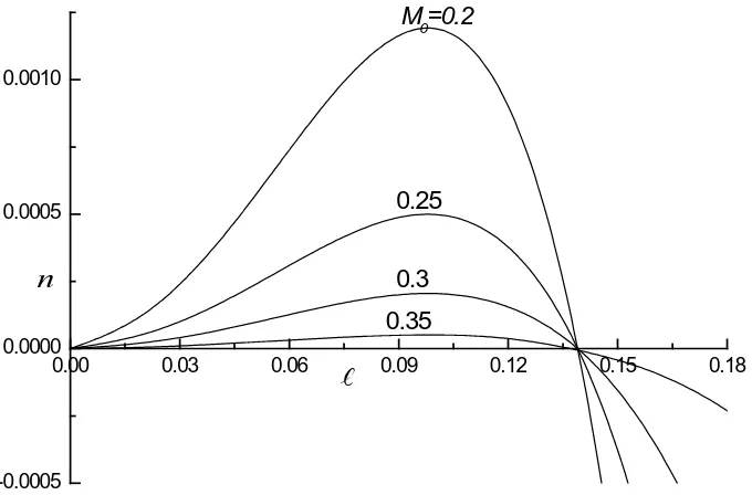
Figure 3. Growth rate, n versus the wavenumber,  for different values of Couple-stress para-meter M0 when αp=0.1,σp=4,B=0.02 and M =5.

0.00 0.03 0.06 0.09 0.12 0.15 0.18

-0.0005 0.0000 0.0005 0.0010

n



0.35 0.3 0.25

[image:8.595.206.546.449.673.2]

[image:9.595.199.552.70.259.2]

Figure 4. Growth rate, n versus the wavenumber,  for different values of Bond number B,

when αp=0.1,σp=4,M0=0.3 and M=5.

0.06 0.09 0.12

0.00008 0.00010 0.00012 0.00014 0.00016 0.00018

0.00020 ₁₀₀

50

20

p

σ =

n



Figure 5. Growth rate, n versus the wavenumber,  for different values of porous parameter

p

σ when αp=0.1,M0=0.3,B=0.02 and M=5.

4. Results and Discussion

In this study we have shown the effect of physical parameters involved in the problem on effect of magnetic field on surface instability of KH type in a couple- stress fluid lay-ers bounded above by a porous layer and below by a rigid boundary. Numerical calcu-lations were performed to determine the growth rate at different wavenumbers for var-ious fluid properties like couple stress parameter M0, Hartmann number M, Bond

0.00 0.05 0.10 0.15 0.20

-0.0002 0.0000 0.0002 0.0004

n



0.01

0.02

[image:9.595.198.550.306.560.2]

number B and porous parameter σp. We have plotted the dimensionless growth rate

of the perturbation against the dimensionless wavenumber for some of the cases only. In the linear stage, all perturbed values grow exponentially in agreement with the dis-persion relation Equation (3.9). At this stage the interface between the layers acquires a sinusoidal shape of small amplitude.

We have investigated the role of the magnetic field on the two-layer channel flow problem, demonstrated that either destabilization or stabilization can be obtained and presented growth rates in situations where the magnetic field is stabilizing over a broad range of wavenumbers for increasing in Hartmann number M in Figure 3 where

0.1, 4, 0.02

p p B

α = σ = = and M0=0.3. The increasing the Hartmann ratio results in

slightly increasing the critical wavenumber and decreasing the maximum growth rate. It thus has a stabilizing effect for the selected values of input parameters due to the in-creased in Hartmann ratio (Lorentz force to viscous force).

Also, when fix all the input parameters we find that the higher the couple-stress pa-rameter the more stable the interface is. In Figure 2, we have plotted the growth rate against the wavenumber in the case where αp =0.1,σp =4,B=0.02 and M =5 for

different values of the couple-stress parameter M0. Increasing the couple-stress ratio

results in slightly increasing the critical wavenumber and decreasing the maximum growth rate this is because of the action of the body couples on the system. Thus, it has a stabilizing effect for the selected values of input parameters due to the increased in the couple-stress parameter.

In addition, we have investigated the effect of the surface tension of the fluid on the instability of the interface. In our sample calculations, we have taken α =p 0.1, M =5,

0 0.3

M = and σ =p 4 and varied the Bond number B. For this input parameters, the

critical wavenumber and maximum growth rate decreased as the ratio of the Bond number B decreased from 0.4 to 0.1 as observed in Figure 4. The Bond number is reci-procal of surface tension and thus showing that an increase in surface tension decreases the growth rate and hence make the interface more stable.

However, in order to understand the effect of the porous properties on the instability, we now fix values of other parameters α =p 0.1, B=0.02, M0=0.3 and M =5

and vary the ratios of the porous parameters. Figure 5 displays the results of our calcu-lations, showing that increasing the ratio of porous parameters σp from 20 to 100 (and

thus increasing the Darcy resistance compared to the viscous force) increases the criti-cal wavelength and decreases the maximum growth rate, thus having a stabilizing effect by this parameter. We conclude that an increase in σp also stabilizes the KHI due to

the resistance offered by the solid particles of the porous layer to the fluid.

5. Conclusions

equations we can analytically predict onset of instability and wavelength for inviscid flow.

We have studied the linear stability of a two-fluid flow in a channel where the fluids are assumed to be Newtonian with different fluid properties (Hartmann number, couple-stress ratio, Surface tension and porous parameter) and subjected to magnetic field normal to their interface. For this purpose, we have derived and then linearized the equations of motion where the interaction between the hydrodynamic and couple- stress problems occurs through the stress balance at the fluid interface. The growth rate of the perturbation was then computed by using the normal mode method and its vari-ation studied as a function of the dimensionless parameter Hartmann number M, couple-stress parameter M0, as well as Bond number B and porous parameter σp.

While two layer flows in channels of small dimensions are rather stable, the instability of the fluid-porous interface is highly desirable in certain cases, particularly for chemi-cal industry, in petroleum production engineering applications where the mixing of reagents are crucial steps in the process. However, in systems of larger scale, the insta-bility of the fluid-porous interface in a channel is often an undesired physical pheno-menon. In such situations, controlling the flow requires the stabilization of the interface. In searching for a method capable of either stabilizing a potentially unstable interface or destabilizing a potentially stable one, we have investigated the role of the magnetic field on the two-layer channel flow problem, demonstrated that either destabilization or stabilization can be obtained and presented growth rates in situations where the mag-netic field is stabilizing over a broad range of wavenumbers for increasing in Hartmann number M as same behavior observed by varying the couple-stress parameter. But in the case of variation in Bond number is to increase in surface tension decreases the growth rate and hence make the interface more stable. Also we conclude that the in-crease in the porous parameter is to dein-crease the growth rate showing thereby the stabi-lizing effect on the interface.

Acknowledgements

This work is supported by the VGST, Department of Science & Technology, Govern-ment of Karnataka under grant no. VGST/SMYSR(2014-15)/GRD-433/2015-16, Dated : 28.04.2015 and the authors (NNK, VBA and PMG) wishes to thank respectively the Di-rector/VC/Principal of their institutions for their encouragement and support in doing research.

References

[1] De Silva, I.P.D., Fernando, H.J.S., Eaton, F. and Hebert, D. (1996) Evolution of Kelvin- Helmholtz Billows in Nature and Laboratory. Earth and Planetary Science Letters, 143, 217- 231. http://dx.doi.org/10.1016/0012-821X(96)00129-X

[2] Von Helmholtz, H.L.F. (1868) Uber discontinuierliche Flüssigkeitsbewegungen.

Monatsbe-richte der königl. Akad. der Wissenschaften zu Berlin, 215-228.

[4] Lamb, H. (1945) Hydrodynamics. 6th Edition, Dover Publications, New York, 738 p. [5] Turner, J.S. (1973) Buoyancy Effects in Fluids. Cambridge University Press, Cambridge, 368

p. http://dx.doi.org/10.1017/CBO9780511608827

[6] Kundu, P.K. (1990) Fluid Mechanics. Academic Press, Cambridge, 638 p.

[7] Scorer, R.S. (1997) Dynamics of Meteorology and Climate. John Wiley & Sons, Hoboken, 686 p.

[8] Chandrasekhar, S. (1961) Hydrodynamic and Hydromagnetic Stability. Oxford University Press, New York.

[9] Malik, S.K. and Singh, M. (1988)Nonlinear Focusing and the Kelvin-Helmholtz Instability in Ferrofluid/Nonmagnetic Fluid Systems. Physics of Fluids, 31, 1069.

http://dx.doi.org/10.1063/1.867018

[10] El-Dib, Y.O. (1996) Nonlinear Stability of Kelvin-Helmholtz Waves in Magnetic Fluids Stressed by a Time-Dependent Acceleration and a Tangential Magnetic Field. Journal of Plasma Physics, 55, 219. http://dx.doi.org/10.1017/S0022377800018808

[11] El-Sayed, M.F. (2002) Effect of Variable Magnetic Field on the Stability of a Stratified Ro-tating Fluid Layer in Porous Medium. Czechoslovak Journal of Physics, 50, 607.

http://dx.doi.org/10.1023/A:1022854217365

[12] Bhatia, P.K. and Sharma, A. (2003) KHI of Two Viscous Superposed Conducting Fluids.

Proceedings of the National Academy of Sciences, India, 73, 497.

[13] Babchin, A.J., Frenkel, A.L., Levich, B.G. and Shivashinsky, G.I. (1983) Nonlinear Satura-tion of Rayleigh-Taylor Instability in Thin Films. Physics of Fluids, 26, 3159.

http://dx.doi.org/10.1063/1.864083

[14] Rudraiah, N., Mathad, R.D. and Betigeri, H. (1997) The RTI of Viscous Fluid Layer with Viscosity Stratification. Current Science, 72, 391.

[15] El-Dib, Y.O. and Matoog, R.T. (2005) Electrorheological Kelvin-Helmholtz Instability of a Fluid Sheet. Journal of Colloid and Interface Science, 289, 223-241.

http://dx.doi.org/10.1016/j.jcis.2005.03.054

[16] Chavaraddi, K.B., Awati, V.B. and Gouder, P.M. (2015) Effect of Surface Roughness on Kelvin-Helmholtz Instability in Presence of Magnetic Field. International Journal of Engi-neering Sciences & Research Technology (IJESRT), 4, 525-534.

Submit or recommend next manuscript to SCIRP and we will provide best service for you:

Accepting pre-submission inquiries through Email, Facebook, LinkedIn, Twitter, etc. A wide selection of journals (inclusive of 9 subjects, more than 200 journals)

Providing 24-hour high-quality service User-friendly online submission system Fair and swift peer-review system

Efficient typesetting and proofreading procedure

Display of the result of downloads and visits, as well as the number of cited articles Maximum dissemination of your research work