Volume 63 Number 6231 DOI: 10.22444/IBVS.6231
Konkoly Observatory Budapest
13 December 2017
HU ISSN 0374 – 0676
SECULAR VARIATION AND PHYSICAL CHARACTERISTICS DETERMINATION OF THE HADS STAR EH Lib
PE ˜NA, J.H.1,2,3; VILLARREAL, C.1,3; PI ˜NA, D.S.1,3; RENTER´IA, A.1,3; SONI, A.3, GUILL´EN,
J.3
& CALDER ´ON, J.1,3
1
Instituto de Astronom´ıa, Universidad Nacional Aut´onoma de M´exico, Cd. M´exico e-mail: [email protected]
2
Observatorio Astron´omico Nacional, Tonantzintla
3
Facultad de Ciencias, Universidad Nacional Aut´onoma de M´exico
1
Motivation
It has been known for quite a while that some high-amplitudeδ Scuti (HADS) stars show long-term variations. In a few cases, after correcting for these long-term variations, the O–C residuals show either sinusoidal variation that can be considered to be due to light-time travel effect provoked by the existence of an unseen companion or, at light-times, show quadratic behavior that is interpreted as secular period variation. With this in mind a search to determine times of maximum light for several HADS stars is being carried out (see Pe˜na et al., 2015) at the Observatorio Astron´omico Nacional de Tonantzintla, M´exico (TNT), an observatory especially suitable for observational teaching practices with small telescopes equipped with modern CCD cameras.
After collecting times of maximum for the HADS stars, a detailed analysis on a star-by-star basis is done. Some results have been published (Pe˜na et al., 2015) and this has stimulated us to study additional stars. These secular variation studies are supplemented withuvby−β photoelectric photometry taken at the Observatorio Astron´omico Nacional de San Pedro M´artir, M´exico (SPM), since the determination of physical parameters of stars can be done through a comparison with theoretical models.
Previous studies on the nature of EH Lib have been extensive. Mahdy & Szeidl (1980) found that this star has a slightly stable, constant period. Jiang & Yang (1981, 1982) obtained six times of maximum that, together with the photoelectric times of maximum compiled over the past 30 years, permitted them to determine the fit with the formula:
Tmax =T0+P0E+
1 2βE
2+Asin 2πEP0
E0
In their article they specified the initial maximum epoch and the pulsation period as
T0 = HJD 2433438.6088 and P0 = 0.0884132445 d, the semi-amplitude and the period of
the sine curve β = −2.8×10⁻⁸ 1/yr; A = 0.0015 d, P
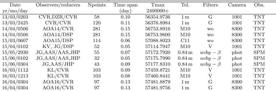
Table 1: Log of observing seasons and new times of maxima of EH Lib.
Date Observers/reducers Npoints Time span Tmax Tel. Filters Camera Obs.
yr/mo/day (day) 2400000+
13/03/0203 CVR,DZR/CVR 58 0.10 56354.9736 1 m G 1001 TNT
13/03/2425 CVR/CVR 120 0.11 56376.8984 1 m G 1001 TNT
14/04/0506 AOA14/CVR 281 0.15 56753.8916 M10 wo 8300 TNT
14/04/0506 AOA14/DSP 281 0.15 56753.9800 M10 wo 8300 TNT
15/03/0607 AOA15/DSP 114 0.06 57088.8023 C11 wo 8300 TNT
15/04/0102 KV, JG/DSP 52 0.05 57114.7947 M10 V 1001 TNT
15/05/2930 JG,AAS/AAS,JHP 55 0.07 57172.7920 0.84 m uvby−β phot SPM 15/06/0102 JG,AAS/AAS,JHP 32 0.05 57175.7990 0.84 m uvby−β phot SPM 15/06/0304 JG,AAS/JHP 43 0.09 57177.8310 0.84 m uvby−β phot SPM
16/03/1112 KL/CVR 103 0.09 57459.8721 M10 V 1001 TNT
16/03/1213 KL/CVR 103 0.08 57460.8441 M10 V 1001 TNT
16/04/0304 AOA16/CVR 97 0.13 57481.8879 1 m G 8300 TNT
16/04/0304 AOA16/CVR 97 0.13 57481.9756 1 m G 8300 TNT
NOTES: CVR, C. Villarreal; DZR, D. Zu˜niga; KV, K. Vargas); DSP, D. S. Pi˜na; JHP, J.H. Pe˜na; AAS, A.A. Soni; JG, J. Guill´en; KL, K. Lozano; AOA14: J. Camargo, O. D´ıaz, J. Flores, D. Galicia, C. Garc´ıa, J. Guill´en,
A. Mu˜noz, M. Paniagua, E. P´erez, J. Ram´ırez, D. S. Pi˜na, M. Serratos, R. Yslas, J. Zamarr´on; AOA15: U. Arellano, J. Diaz, I. Fuentes, A. Mata, I. Mora, X. Moreno,F. Ruiz, K. Valencia, K. V´argas; AOA16: K. Ju´arez,
K. Lozano, A. Padilla, R. Vel´azquez, P. Santill´an. C11: 11” Celestron, M10: 10” Meade telescopes.
number of periods elapsed since T0, and E0 = 70700, which can be interpreted as a 17.1
year periodicity as a modulation of the phase of maximum by binary motion.
More recently, Joner (1986), with uvby−β photometry determined a reddening value of E(b−y) = 0.041, a mean effective temperature of Teff = 7840 K and a mean surface
gravity, log g = 4.08. The metal abundance, [Fe/H] =−0.015 was also determined. Using a Wesselink method they derived a mean radius of 2.4 R⊙, a mean absolute bolometric
magnitude of Mbol = +1.5 mag, and a mass of 2.0M⊙.
In their study devoted to EH Lib, Wison et al. (1993) stated that it was a large-amplitude δ Sct variable star and that it had a range of 9.35−10.08 mag in V and a spectral class range A5–F3 according to the General Catalogue of Variable Stars (Baker, 1985).
McNamara and Feltz (1976) obtained a Wesselink radius of 2.1R⊙, but did not discuss
the uncertainty in the result. Later, McNamara and Feltz (1978) used the observed effective gravities of 15 dwarf Cepheids, as they were known at that time, including EH Lib, to derive an empirical equation relating radius R to period P. They proposed the relation: log R = 0.80 logP + 1.17. They also commented that according to Joner (1986), a mean value of 2.4R⊙for the Wesselink radius was found from the values derived
for the effective temperature (Teff) as a phase function from uvby −β photometry. The
radial-velocity measurements were taken from photographic spectrograms.
2
Observations
2.1 Data acquisition and reduction in TNT
During all the observational nights the following procedure was utilized. Sequence strings were obtained: the integration time for the 1 m telescope (in the G filter) was 3 min and that of the smaller telescopes (in the V filter) was shorter (1 min). It may seem contradictory to give a longer integration time to the larger aperture telescope, however, this was done since the mounting of the smaller telescopes is alt/az which does not allow long integration times. Nevertheless, for the 1 m telescope there were around 40,000 counts and for the 10” and 11” telescopes there were 11,000 counts, enough to secure high
precision. The reduction work was done with AstroImageJ (Collins, 2012), a software that is relatively easy to use and has the advantage that it is free and works satisfactorily on the most common computing platforms. With the CCD photometry two reference stars were utilized whenever possible in a differential photometry mode. The results were obtained from the difference Vvar −Vref and the scatter calculated from the difference
Vref1−Vref2. This scatter is 0.03941 mag. The times of maxima were easily determined
by fitting a fifth-degree polynomial.
2.2 Data acquisition and reduction in SPM
The 0.84 m telescope to which a spectrophotometer was attached was utilized at all times. The observing season lasted six nights from May–June 2015 but only three were devoted to the observation of EH Lib (which were done by A. A. Soni & J. Guillen). The observation and reduction procedures have been extensively utilized. See for example Pe˜na et al. (2016).
The coefficients defined by the following equations with the data adjusted to the stan-dard system are:
Vstd = 17.6893 + 0.0340(b−y)inst+yinst
(b−y)std = 1.4055 + 0.9692(b−y)inst
m1std = −1.3713 + 1.0928(m1)inst+ 0.0134(b−y)inst
c1std = 0.0419 + 1.0341(c1)inst+ 0.1392(b−y)inst
Hβstd = 2.3513 +−1.3565(Hβ)inst
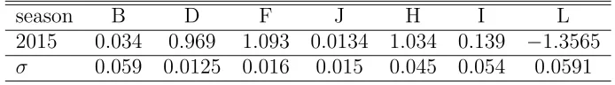
The averaged transformation coefficients of each night are listed in Table 2 along with their standard deviations. In these equations the coefficients D, F, H and L are the slope coefficients for (b−y), m1, c1 and β. The coefficients B, J and I are the color terms of
V, m1, and c1. Season errors were evaluated using the standard stars observed. These
uncertainties were calculated through the differences in magnitude and colors, for (V,
b−y, m1, c1 and β) as (0.0361, 0.0119, 0.0150, 0.0197, 0.0213), respectively, providing
a numerical evaluation of our uncertainties. Emphasis is made on the large range of the standard stars in the magnitude and color values: V:(5.2, 8.8); (b−y):(-0.01, 0.79);
m1:(0.09, 0.70);c1:(0.23, 1.39) andβ:(2.52, 2.90).
Table 2: Transformation coefficients obtained for the observed season.
season B D F J H I L
2015 0.034 0.969 1.093 0.0134 1.034 0.139 −1.3565
σ 0.059 0.0125 0.016 0.015 0.045 0.054 0.0591
3
Period determination
3.1 Time series analysis
As in the case of AE UMa (Pe˜na et al., 2016), we were lucky to have previously reported observations of EH Lib in Str¨omgren photometry. There are three samples: the data presented by Epstein (1969) in ubvy only, that of Joner (1986) and that of the present paper with data from 2015 in uvby − β photometry. The question that immediately arises relates to the concordance of these three samples. A phase diagram was built considering alluvby−βdata with the latest period analysis and the ephemerides elements of Boonyarak et al. (2011), it is shown in Figure 1. What is immediately seen from this figure is that: i) the phase concordance of the three samples implies a constant period for at least the time span of 47 years and ii) there is a large dispersion in the m1 and β
indexes.
To determine the period, at this stage, we will consider only the V magnitude which has a remarkable good behavior given the long time separation of the sets, with only very few discordant points that were discarded. We were left with a set of 264 data points in this V filter.
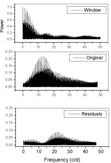
With such a long time basis in the uvby−β time series, a period can be determined through Fourier transforms. As with the short period variable community we utilized Period04 (Lenz & Breger, 2005) with a frequency interval between 0 and 50 c/d. The window pattern is complex due to the scarce and separated data sets. Figure 2 schemat-ically shows the obtained results. The frequency spectrum of the original data presents a peak at 12.3132578±0.5×10⁻⁶ c/d with an amplitude of 0.212±5×10⁻³ mag and
a phase of 0.241±4×10⁻³. The uncertainty was evaluated by the method included in
Period04.
The second highest point is at 11.3106898 c/d which corresponds to the period proposed by Boonyarak et al. (2011) of 0.08841326 d. However, when this maximum is enlarged it unfolds into two close maxima at 11.3106898 c/d and 11.3108600 c/d of amplitude of the same order. If the first case is analysed for the residuals, a peak at 23.6246307±2×10⁻⁶
c/d is obtained which is merely a 2f value of the determined frequency. The amplitude which corresponds to this is 0.083±6×10⁻³ mag with a phase of 0.55±1×10⁻². The
analysis of the residuals of these two frequencies yields a peak at 32.9192025±3×10⁻⁶
c/d with an amplitude of 0.040±4×10⁻³ mag and a phase of 0.22±1×10⁻². Again,
the predictions versus the observations show a remarkable fit.
Figure 1. Phase plot of theuvby−β photometry of Epstein (1969), Joner (1986) and the present paper. The time span between these sets is 49 years. The period considered is that proposed by
Boonyarak (2011).
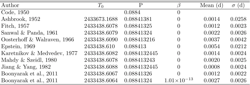
[image:5.595.205.382.459.719.2]Table 3: EH Lib ephemeris equations.
Author T0 P β Mean (d) σ(d)
Code, 1950 0.0884 0
Ashbrook, 1952 2433673.1688 0.08841381 0 0.0014 0.0258
Fitch, 1957 2433438.6078 0.08841325 0 0.0012 0.0023
Sanwal & Panda, 1961 2433438.6079 0.08841324 0 0.0022 0.0026 Oosterhoff & Walraven, 1966 2433438.6090 0.088413216 0 0.0037 0.0042
Epstein, 1969 2433438.610 0.088413 0 0.0054 0.0212
Karetnikov & Medvedev, 1977 2433438.6082 0.0884132445 0 0.0014 0.0024 Mahdy & Szeidl, 1980 2433438.6078 0.088413243 0 0.0020 0.0025 Jiang & Yang, 1982 2433438.6088 0.0884132445 0 0.0008 0.0024 Boonyarak et al., 2011 2433438.6067 0.08841326 0 0.0012 0.0022 Boonyarak et al., 2011 2433438.6064 0.08841324 1.01×10⁻¹³ 0.0027 0.0026
3.2 O–C analysis
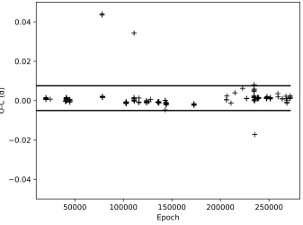
As a first step in carrying out an analysis of the secular variation, an O–C vs. epoch a diagram was constructed with all the compiled times of maximum light. Taking the most recent reported analysis (Boonyarak et al., 2011) we obtained the O–C residuals shown in Figure 3. Only a very few points (five) were outside the standard deviation limits. Hence these points were discarded in the subsequent analyses. Numerically, this is equivalent to adjusting a Gaussian to the O–C residuals and discarding those points beyond one sigma. The limit in this case is 0.0054.
The whole sample of 237 times of maximum covering a time span of 66 years was employed as a first step to determine the behavior of EH Lib. New times of maximum considered after the analysis of Boonyarak et al. (2011) were reported in H¨ubscher et al. (2009, 2013), Wils et al. (2011, 2012) and this paper all gathered from 2013 to 2016. In two of the papers utilized in our compilation (Pohl 1955, H¨ubscher et al. 2013), several of the maximum times were observed simultaneously by different observers and included independently in the same paper, so we made an average of these apparently repeated data. Since the times of maximum in the paper by Karetnikov (1977) had no heliocentric correction, we added it and these points are included in our compilation, but not in the analysis. After these procedures there were 226 times of maximum left.
50000 100000 150000 200000 250000 Epoch
−0.04 −0.02 0.00 0.02 0.04
O
-C
(
[image:7.595.117.454.120.370.2]d)
Figure 3. O–C diagram with all the measured times of maximum light.
3.3 Minimization of the standard deviation of the O–C residuals (MSDR)
To determine the ephemerides equation of the variability of EH Lib we, as was previ-ously mentioned, omitted the visual and photographic points and made use of only the photoelectrical ones.
To calculate the ephemerides equation, a standard deviation minimization of the O– C diagram was built. The standard deviation of several O–C diagrams for this same star was calculated. In all cases, as a first step in constructing these O–C diagrams, T0
and the period P were used as the first time of maximum with each one of the points between 0.087251454 and 0.089596791 with a precision of 1×10⁻⁹. This range is the one
provided by the average of the difference of consecutive times of maximum light and the standard deviation of the same. With all of the 2345336 periods, the cycle number E of all the times of maximum was calculated. The second step was to make a linear fit of the times of maximum with the cycle number (HJD vs. E) for each different period in the range. The new periodP and initial epoch T0 were obtained and are the parameters
of the ephemerides equation needed to construct the O–C diagrams. These linear fits were carried out 2345336 times. Finally, the period and initial epoch with the smallest standard deviation of its O–C diagram was selected as the best equation. The result of these calculations is shown graphically in Figure 4. The O–C diagram obtained with this method is presented in Figure 5 and its equation is:
Tmax = 2435223.7584 + 0.088413266E
Figure 4. Standard deviation vs. Period of the standard deviation minimization of the O–C residuals method in the linear case.
0 50000 100000 150000 200000 250000 Epoch
−0.0100 −0.0075 −0.0050 −0.0025 0.0000 0.0025 0.0050 0.0075 0.0100
O
-C
(
d)
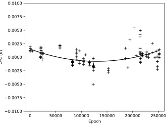
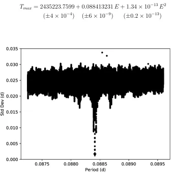
[image:8.595.119.454.469.724.2]A parabolic trend is present in the O–C diagram as can be seen in Figure 5. To be able to get the parameters of that second order changing period, we followed the same method but instead of fitting the data to a straight line, it was fitted to a parabola. The standard deviation vs. period diagram using the parabolic fit is shown in the Figure 6. The result of subtracting this parabolic trend from the data is shown in the Figure 7. The parabolic equation is:
Tmax = 2435223.7599 + 0.088413231E+ 1.34×10
−13E2
[image:9.595.116.454.173.514.2](±4×10−4) (±6×10⁻⁹) (±0.2×10⁻¹³)
Figure 6. Standard deviation vs. period of the standard deviation minimization of the O–C residuals method in the quadratic case.
4
Determination of physical parameters
To determine the physical characteristics of the star, we first evaluated the reddening through Str¨omgren photometry and the appropriate unreddening calibrations. As was mentioned before, there are three samples of data with uvby −β photometry: that of Epstein (1969) in ubvy only; that of Joner (1986), and that present in the online data table which was taken in 2015. A phase diagram was built considering all uvby−β data with the ephemerides elements of Boonyarak et al. (2011) and it is shown in Figure 1. A phase concordance within the three samples implies a constant period for at least 47 years although there is a large dispersion in them1andβindexes. The physical parameter
0 50000 100000 150000 200000 250000 Epoch
−0.0100 −0.0075 −0.0050 −0.0025 0.0000 0.0025 0.0050 0.0075 0.0100
O
-C
(
[image:10.595.118.454.118.369.2]d)
Figure 7. O–C Diagram of EH Lib calculated with the ephemerides equation obtained with the MSDR method in the quadratic case.
reddening, and hence the unrreddened color indexes for the late A and F stars to which EH Lib belongs. Values of reddening, unreddened indexes, absolute magnitude, distance modulus, distance and metallicity were determined through the mathematical expressions proposed by Nissen (1988, his equations 3, 4, and 10), which can be used to calculate the intrinsic color index (b−y)0. The absolute magnitude was then calculated for A and F
type stars whereas the metallicity (Nissen 1988, his equations 6, 7, and 8) is determined only when the star is in its F stage.
To avoid large dispersion in the output values due to the large scatter of the m1
values caused by a noisyu filter, mean values for each index and physical parameter were calculated in phase bins of 0.05. The results of using the above mentioned prescriptions are listed in Table 4 in increasing phase values column 1 lists the mean bin values, and the following columns list the reddening E(b−y), the values for the unreddened (b−y)0,
the m0, the c0, the β, the Mv indexes.
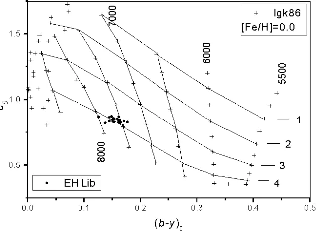
To determine the physical characteristics of the star, these phase averaged, unreddened values were plotted in a (b−y)0 vsc0 grid and overlapped with those values calculated by
Lester et al.(1986, hereinafter LGK86) for theoretical uvby−β indices. The comparison is presented in Figure 8 from which we find the limits of variation of EH Lib in bothTeff
Table 4: Reddening and unreddened values ofuvby−β photometry for EH Lib.
Phase E(b−y) h(b−y)0i hm0i hc0i β Mv
0.05 0.006 0.157 0.177 0.851 2.778 1.7 0.15 0.002 0.122 0.179 0.953 2.809 1.3 0.25 0.001 0.127 0.175 0.968 2.801 1.1 0.35 0.005 0.145 0.171 0.920 2.784 1.3 0.45 0.007 0.159 0.169 0.871 2.772 1.5 0.55 0.002 0.180 0.166 0.833 2.751 1.5 0.65 0.002 0.197 0.167 0.788 2.734 1.6 0.75 0.005 0.201 0.165 0.768 2.732 1.8 0.85 0.006 0.199 0.163 0.763 2.735 1.9 0.95 0.004 0.184 0.170 0.776 2.752 2.1
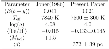
Table 5: Physical parameters determination throughuvby−β photometry for EH Lib.
Parameter Joner(1986) Present Paper
hE(b−y)i 0.041 0.021
Teff 7840 K 7500 ± 300 K
log(g) 4.08 4.0
h[Fe/H]i −0.015 −0.133±0.145
hMboli +1.5
hdi 372 ± 39 pc
5
Discussion
In previous research, Boonyarak et al. (2011) reported 0.0033 days as the RMS of the residuals of linear and quadratic fits and a period variation rate of (9.44×10⁻⁹) per year.
Jiang & Yang (1982) used yearly averaged times of maximum light to study the period variations and found a light time effect. They stated that 29 years later the phenomenon was not shown clearly in the direct (O–C) distribution but the light time effect was still visible if the yearly average was used again.
Wilson et al. (1993) calculated the phase using Jiang and Yang’s (1982) elements
E0 = 2433438.6082 and E0 = 2433438.6082, but they reported that they didn’t have
enough high precision data to test the hypotheses of either a possible binary orbital motion or a Blazhko effect (Karetnikov & Medvedev, 1979) due to the low amplitude of the effects.
[image:11.595.185.412.348.451.2]Figure 8. Cycle variation of EH Lib in the theoretical grids of LGK86.
obtaining a flattened O–C diagram in the residuals.
Mahdy and Szeidl (1980) affirmed a constant period, which was correct at that time; but after 36 years of further observations we can see a more complete behavior. Even with the 5 additional years to the Boonyarak et al. (2011) data base, the parabolic behavior is clearly discernable.
For the physical parameters the following is stated: uvby−β photoelectric photometry was previously obtained for EH Lib by Epstein (1969) and by Joner (1986). From anal-ogous considerations as those taken in the present paper they derived their own physical parameters. These are presented in Table 4.
6
Conclusions
Thirteen new times of maximum have been gathered for the HADS star EH Lib from two observatories with CCD and uvby−β photometry. From theuvby−β data, physical parameters were determined and were utilized to obtain the period of the star. The use of two more samples of uvby−β photometry previously obtained allowed us to extend the time basis to a time span of 49 years. A minimization of the standard deviation of the O–C residuals was performed to determine the best parameters for the ephemerides equations of EH Lib and a long-term secular variation was found. The physical parameters provided by the present paper are in agreement with those of Joner (1986).
observations. Typing and proofreading were done by J. Orta, and J. Miller, respectively. C. Guzm´an, F. Salas and A. Diaz assisted us in the computing. This research has made use of the Simbad databases operated at CDS, Strasbourg, France and NASA ADS Astronomy Query Form.
References:
Ashbrook, J., 1952,AJ,57, Q64 DOI Baker, N. H., 1985, IBVS, 2709
Boonyarak, C., Fu, J. N., Khokhuntod, P., & Jian, S., 2011, ApSS, 333, 125 DOI Code, A. D., 1950, PASP, 62, 166 DOI
Collins, K., 2012, Astronomy Source Code Library, 1309.001 Epstein, I., 1969,AJ,74, 1131 DOI
Fitch, W. S., 1957, AJ, 62, 108 DOI H¨ubscher, J. et al., 2009, IBVS, 5889 H¨ubscher, J. et al., 2013, IBVS, 6048
Jiang, S. Y. & Yang, Z. Z., 1981,Acta Astronomica Sinica,22, 279
Jiang, S. Y. & Yang, Z. Z., 1982,Chinese Astron. & Astrophys., 6, 24 DOI Joner, M. D., 1986, PASP, 98, 651 DOI
Karetnikov, V. G. & Medvedev Yu., 1977,IBVS, 1310 Karetnikov, V. G. & Medvedev, Yu. A., 1979, IBVS, 1537 Lenz, P. & Breger, M., 2005, CoAst, 146, 53 DOI
Lester, J. B., Gray, R. O. & Kurucz, R. I., 1986,ApJS, 61, 509 DOI Mahdy, H. A. & Szeidl, B., 1980, CoKon,74, 1
McNamara, D. & Feltz, K. A., 1976,PASP,88, 164 DOI McNamara, D. & Feltz, K. A., 1978,PASP,90, 275 DOI Nissen, P., 1988, A&A,199, 146
Oosterhoff, P.Th. & Walraven, Th., 1966, BAN, 18, 387
Pe˜na, J. H., Renteria, A., Villarreal, C. et al., 2015, IBVS, 6154
Pe˜na, J. H., Villarreal, C. Pi˜na, D. S. et al., 2016,RevMexAA, 52, 385 Pohl, E. 1955, AN, 282, 235 DOI
Sanwal, N. B. & Pande, M. C., 1961, Observatory, 81, 199 Wils, P. et al. 2011,IBVS, 5977
Wils, P. et al. 2012,IBVS, 6015