The Suitable Power Control of Wind Energy Conversion
System based doubly Fed Induction Generator
K D E. Kerrouche
Department of Electrical Engineering, Faculty of sciences Engineering Tahar
Moulay University, SAIDA, Algeria
A. Mezouar
Department of Electrical Engineering, Faculty of sciences Engineering Tahar
Moulay University, SAIDA, Algeria
L. Boumedien
Department of Electrical Engineering, Faculty of sciences Engineering Tahar
Moulay University, SAIDA, Algeria
ABSTRACT
The aim of this paper is to propose different methods of control for a Doubly-Fed Induction Generator (DFIG) used in wind energy conversion systems. This paper presents a comparative study on the performance of three control methods for DFIG wind turbine. The study focuses on the regulation of the active and reactive power exchanged between the generator and the grid by the generator inverter using the control algorithm based on vector control concept (stator flux orientation), with classical PI controllers: proportional–integral. The different methods of control for the generator are simulated in MATLAB / SIMULINK and discussed. Therefore, we conclude which is a suitable control of DFIG in Wind Energy Conversion System.
Keywords
Doubly fed induction generator, stator flux orientation, Power control
1.
INTRODUCTION
Wind energy is one of the most promising renewable energy sources due to the progress experienced in the last decades. Governments are attracted by the Wind Energy Conversion System (WECS) with its simple structure, easy maintenance and management. With an average global annual growth rate of 14% for the period 2002-2006. Wind energy is playing a major role in the effort to increase the share of renewable energy sources in the world energy mix [1], [2], helping to satisfy global energy demand, offering the best opportunity to unlock a new era of environmental protection [3], the world energy crises can be solved in future.
DFIG has recently received much attention as one of preferred technology for wind power generation. Compared to a full rated converter system, the use of DFIG in a wind turbine offers many advantages, such as reduction of inverter cost, the potential to control torque and a slight increase in efficiency of wind energy extraction. The wind turbines variable-speed operation has been used for many reasons. Among these are the decrease of the stresses on the mechanical structure, acoustic noise reduction and the possibility of active and reactive power control [1]. Most of the major wind turbine manufacturers are developing new larger wind turbines in the
[5]; this means that the losses in the power electronics converters, as well as the costs, are reduced.
Motivated by the reason above, this paper provides a study of the dynamics of the grid connected wind turbine with DFIG.
Many papers have been presented, with different control schemes of WT to extract a maximum power from wind speed variable, based on fuzzy controller as it is commonly done in literature [1, 2 and 3]. The DFIG control schemes are generally based on vector control concept (with flux orientation) with Sliding Mode Control (SMC) as proposed in [4]. SMC of Active and Reactive Power of a DFIG and extracting maximum power for Variable Speed by WECS in [5, 6]. Many works are done about decoupled control of DFIG to improve power quality for WECS. In [7, 8] have studied an advanced control of DFIG and power quality improvement. In [9] a comparison of FACTS devices like STATCOM and SVC for the voltage stability issue for IG-based wind farm connected to a grid and load.
This paper presents a three control methods for the generator inverter in order to regulate the active and reactive power exchanged between the machine and the grid. Such an approach can manage easily the compromise between dynamic performances and robustness or between dynamic performances and the generator energy cost. These compromises can easily be respected with classical PI controllers in DFIG control schemes proposed in this paper.
The paper is organized as follows: section II presents the entire system model under study. The three control strategies of DFIG and the design of the PI controller are dealt, and then are applied in section III. In section V, some results of simulations, to validate the proposed DFIG control framework are presented and discussed. Section VI concludes the paper.
2.
MODELING OF WECS CHAIN
Fig 1: Wind energy conversion chain.
2.1
Modeling of the turbine and the
gearbox
Wind turbine generation systems’ (WTGS) convert power from the kinetic energy of the wind, thus it can be expressed as the kinetic power available in the stream of air multiplied by a Cp factor called power coefficient or Betz’ s factor. The aerodynamic power is given by:
3
)
,
(
2
1
SV
C
P
t
p
(1) Where
is the air density,R
is the blade length andV
the wind velocity.A wind turbine can only convert just a certain percentage of the captured wind power. This percentage is represented by
) ( p
C which is function of the wind speed, the turbine
speed and the pith angle of specific wind turbine blades [5], [6]. Although this equation seems simple, Cpis dependent on the ratio between the turbine angular velocity
t and the wind speedV
. This ratio is called the tip speed ratio:V
R
t
(2)
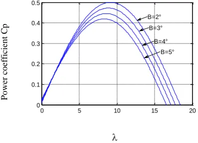
The typical Cp versus curve is shown in Fig.3. In a wind turbine, there is an optimum value of tip speed ratio for which
p
C is maximum and that maximises the power for a given
wind speed. The peak power for each wind speed occurs at the point where Cp is maximised. To maximise the generated power, it is therefore desirable for the generator to have a power characteristic that will follow the maximum Cpmax line [7].
A figure showing the relation betweenCp,
and
is shown in Fig. 2.P
o
we
r
co
efficie
n
t
C
p
Fig 2: Power coefficient variation against tip speed ratio and pitch angle.
The turbine torque is the ratio of the output power to the shaft
speed
t,t t aer
P
T
The turbine is normally coupled to the generator shaft through a gearbox whose gear ratio
G
is chosen in order to set the generator shaft speed within a desired speed range. Neglecting the transmission losses, the torque and shaft speed of the wind turbine, referred to the generator side of the gearbox, are given by:
G G T T
m t
aer g
(3)
WhereTg the driving torque of the generator and
mis the generator shaft speed, respectively.2.2
Modelling of the DFIG
A typical configuration of a DFIG wind turbine is shown in Fig1. It uses a wound-rotor induction generator with slip-rings to transmit current between the converter and the rotor windings and variable-speed operation is obtained by injecting a controllable voltage in to the rotor at the desired slip frequency. It is used to produce electrical power at constant frequency whatever wind and shaft speed conditions. The rotor winding is fed through a variable-frequency power converter, typically based on two AC/DC IGBT-based Voltage Source Converters (VSCs), and linked through a DC bus. The variable- frequency rotor supply from the converter enables the rotor mechanical speed to be decoupled from the synchronous frequency of the electrical network, there by allowing variable-speed operation of the wind turbine [10].
The equations for a DFIG are identical with a squirrel-cage induction generator except that the rotor voltages are not zeros. Using faraday’s law and ohm’s law, the expressions relating the voltages with the currents and fluxes across the stator winding in the PARK frame are written as follows[ 11]: Gearbox
Generator
Converter DFIG
Grid
Control Turbine
0 5 10 15 20
0 0.1 0.2 0.3 0.4 0.5
B=2° B=3° B=4°
[image:2.595.321.520.79.222.2] qr s s r dr r r qs s s ds s qr r qs s qr qr r r dr s s r qs s ds s s dr r ds s dr qr s s qs s s ds s qs qs dr s s qs s ds s s ds ds i R L M R i L L R M L M dt di L v L M v i L i R L M R L M L R M dt di L v L M v i L R M L R dt d v i L R M L R dt d v ) ( ) ( 2 2 2 2 2 2
(4)
Where
R
sandR
r are, respectively, the stator and rotorphase resistances.
L
s,L
r,M
Stator and rotor perphase winding and magnetizing inductances.
p
mecis the electrical speed andp
is the pair pole number.The stator and rotor flux can be expressed as:
qs qr r qr ds dr r dr qr qs s sq dr ds s ds Mi i L Mi i L Mi i L Mi i L
(5)
Where
i
ds,iqs,i
dr, andiqr are, respectively, the direct and quadrate stator and rotor currents.The active and reactive powers at the stator, as well as those provide for grid are defined as:
qs ds ds qs s qs qs ds ds si
v
i
v
Q
i
v
i
v
P
(6)
The electromagnetic torque is expressed as:
) (qs ds ds qs
em pi i
T
(7)
3.
POWER CONTROL OF THE DFIG
3.1
Decoupling of the active and reactive
powers
When the DFIG is connected to an existing grid, this connection must be established in the following three steps. The first step is the synchronization of the stator voltages with the grid voltages, which are used as a reference. The second step is the stator connection to this grid. After that, the
0
s ds qs(9)
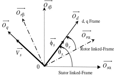
[image:3.595.330.523.133.265.2]In the park reference frame, approach is shown in Fig. 4.
Fig 4: Flux Orientation.
Using the condition above, supposing that the grid system is steady, having a single voltage
V
s that leads to stator’sconstant flux
s, we can easily deduce the voltages as:
s s s qs dsV
v
v
0
(10)
Per phase stator resistance is neglected, which is a realistic approximation for medium power machines used in WECS, the stator voltage vector is consequently in quadrate advance in comparison with the stator flux vector.
By using equations (10) and (4), the rotor voltages are:
s s dr r r qr r qr r qr ds s qr r r dr r dr r drV
L
M
s
i
L
i
R
dt
di
L
v
dt
d
L
M
i
L
i
R
dt
di
L
v
(11)
Where
V
s is the stator voltage magnitude assumed to be constant ands
is the slip range, the rotor voltages are obtained as follows: q qr r qr r qr d dr r dr r dr fem i R dt di L v fem i R dt di L v
(12)
With
fem
d and femq are the crosses coupling terms between thed
axis andq
axis:
femd Lrriqr
Stator linked-Frame r
O
sO
Rotor linked-Frame
qr qs s dr ds s dsMi
i
L
Mi
i
L
0
(14)
From (14), the currents can be deduced as:
qr s qs s dr ds ds i L M i L Mi i
(15)
Using Equations (6), (10) and (15) the stator active and reactive power can then be expressed only versus these rotor currents as:
M
i
L
M
V
Q
i
L
M
V
P
ds dr s s s qr s s s (16)Using (12), (16), the active and reactive power are expressed as:
s ds s d dr r r s s s q qr r r s s s L V fem v R p L L M V Q fem v R p L L M V P 1 1(17)
Field oriented control of the DFIG can then be applied with the active and reactive power considered as variables to be controlled. Without taking into account the transfer function of the inverter used to feed the rotor. We will consider that this inverter dynamic is very fast; it can take a unitary coefficient.
[image:4.595.314.534.83.364.2]The block diagram of the system to be controlled is presented in Fig. 5.
Fig 5: Decoupled model of active and reactive stator powers.
3.2
Direct power control
To realize an electrical production control of WECS, with carrying out a decoupled control of the DFIG active and reactive powers. For this purpose, we should eliminate the cross coupling terms between the d-axis and q-axis by a feed forward compensation. Therefore, we control each power axis separately by adding a PI regulation in the loop. Thus, the powers regulators control directly the machine rotor voltages.
Thereby, this method is called direct power control, as shown in Fig. 6.
Fig. 6: Scheme of direct power control.
3.3
Indirect power control
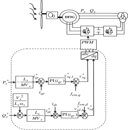
[image:4.595.56.278.494.646.2]The second method takes into account the cross coupling terms and compensates them, with carrying out that the decoupled control which includes two rotor currents loops, which can be controlled by adding a PI regulator in each loop, whose their references are directly deduced from the powers references values, imposed for the machine. Thus, the rotor currents regulators control indirectly the machine rotor voltages, without using a power loop. Thereby, this method is called indirect power control without power loop, as shown in Fig. 7.
Fig 7: Scheme of indirect power control without power loop 1 s
L
rdv
rqv
d emf
, q emf
, s Q sP
s s V
r r
s s
R
p
L
L
M
V
1
r r
s s
R
p
L
L
M
V
1
* s Q s Q * s P s P * 1 , dr v * 1 , qr v * qr v * dr v dq abc s P QsDFIG
PWM
) ( PI Ps
) ( PIQs
d em f , q em f , * s Q * s P * 1 , rq v * rq v * rd v dq abc s
P Qs
DFIG PWM d em f , q em f , s s MV L s s s L V 2 qr i dr i s s MV L * qr i * dr i ) ( PIiqr
) ( PIiqr
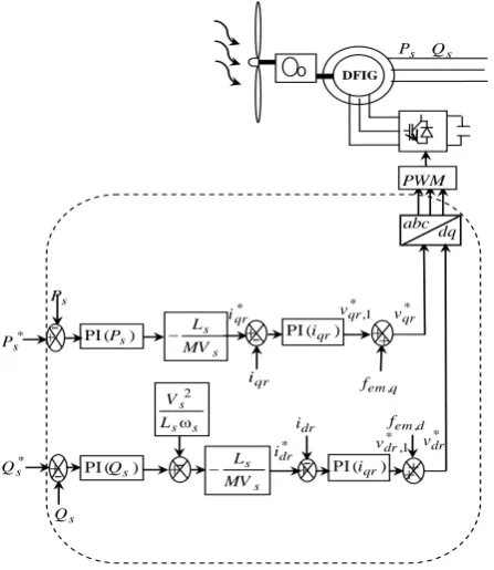
[image:4.595.315.540.499.727.2]To improve the indirect control, we can add a regulation loop of powers to eliminate the static error while maintaining the system dynamics. Therefore, we can distinguish the two regulation loop for each axis using PI regulator, one for controlling current and the other for power. Thereby, this method is called indirect power control with power loop, as shown in Fig. 8.
Fig 8: Scheme of indirect power control with power loop.
3.4
PI controller synthesis
The controller terms are calculated with a pole-compensation method. The time response of the controlled system will be fixed at 10 ms, this value is sufficient for our application and a lower value might involve transients with important overshoots.
It is possible to generate the reference voltages from given reference powers. The design of this controller is simple. Fig. 9 shows the block diagram of the system with PI controller.
Fig 9: Power-control loop.
In fact, the (
P
s*
P
s) and (Q
s*
Q
s) errors are processed by PI controller to give vqrandv
dr.Using the Laplace Transform, the plant can be represented by the Closed Loop Transfer Function (CLTF) below:
With:
r r s
s T T
R L
MV A
[image:5.595.311.542.131.347.2]
The calculated terms are in these tables:
Table 1. The calculated PI gains for the stator active power
s P p
K
,K
i,PsPI controller
(
2
T
1
)
/
A
0
T
2/
A
0
Value -9.1470e-004 0.1185
Table 2. The calculated PI gains for the stator reactive power
s P p
K
,K
i,PsPI controller
(
2
T
0
1
)
/
A
A
T
20/
Value -9.1470e-004 0.1185
It is possible to generate the reference voltages from given reference currents. The design of this controller is simple Fig. 10 shows the block diagram of the system with PI controller.
Fig 10: Current-control loop.
In fact, the (iqr* iqr) and (
i
dr*
i
dr) errors are processed by PI controller to give vqrandv
dr .Using the Laplace Transform, the plant can be represented by the Closed Loop Transfer Function (CLTF) below:
T
K
A
T
K
A
s
s
K
s
K
T
A
CLTF
i p
i p
1
)
(
2
(20)
With:
r r T T
R
A 1
Table 3. The calculated PI gains for the direct axis
id p
K , Ki,id
*
s
Q
*
s
P
* 1 ,
qr
v *
qr
v
*
dr
v
dq abc
s
P Qs
DFIG
PWM
d em
f ,
q em
f ,
s s
MV L
s s
s
L V
2 qr
i
dr
i
s s
MV L
*
qr
i
*
dr
i
) ( PIiqr
) ( PIiqr
*
1 ,
dr
v )
( PIQs
) ( PI Ps
) ( PIQs
s
P
s
Q
* r
v
-
sK
K i
p
+
TsA .
1
s s Q
P , *
* , s s Q P
r v*
-
s
K
K
p,id
i,id* r i
+
T
s
A
.
1
[image:5.595.57.281.150.408.2]Table 4. The calculated PI gains for the quadrate axis
iq p
K , Ki,iq
PI controller
r
r
R
T
1
)
2
(
0
r r
R
T
20
Value 0.0331 3.7576
The pole- compensation in not the only method to calculate PI Controller but it is simple to elaborate with first-order transfer-function and it is sufficient in our case of study.
In fact, the (
P
s*
P
s) and (Q
s*
Q
s) errors are processed by PI controller to give vqrandv
dr. [image:6.595.314.541.73.332.2]Using the Laplace Transform, the plant can be represented by the Closed Loop Transfer Function (CLTF) below:
Fig 11: Power-control loop.
s AK CLTF
i 1 1
1
(21)
With considering
1.0000e
-
004
a time constant, (21) becomes:p
CLTF
1
1
(22)
With:
0 T
L M V A
s
s and
A
K
K
i p
1
0
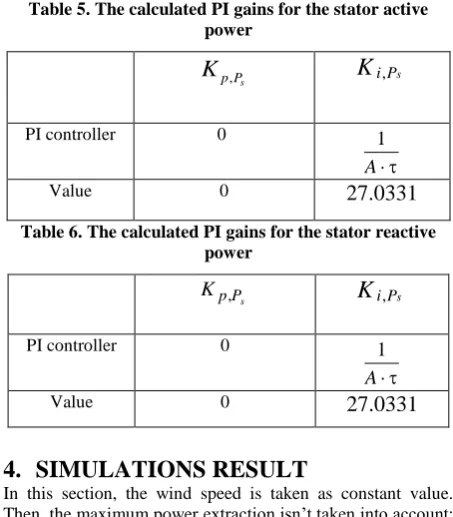
Table 5. The calculated PI gains for the stator active power
s P p
K
,K
i,PsPI controller 0
A 1
Value 0
27.0331
Table 6. The calculated PI gains for the stator reactive power
s
P p
K
,K
i,PsPI controller 0
A 1
Value 0
27.0331
4.
SIMULATIONS RESULT
In this section, the wind speed is taken as constant value. Then, the maximum power extraction isn’t taken into account; the wind turbine is driven around synchronous generator speed (312 rd/s). Besides, the turbine and the generator are considered as working over ideal conditions (no perturbation); their parameters are shown in the appendix.
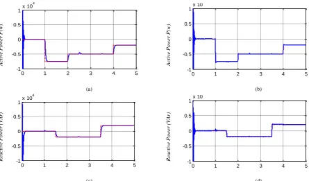
The simulation is performed by imposing the active and
reactive power reference (
P
s*,Q
s*).P
s* range between 0, -7500, -5000 and -2500watts,Q
s* range between 0, -2500 and-2500 VAr.Fig. 12, 13 present the simulation results of the direct control, indirect control without power loop.
s s P Q ,
* *
,, s s P Q
s
Q
+
s s
L
M
V
[image:6.595.56.281.301.422.2]Fig 12: (a) Stator active power of direct control (b) Stator active power of indirect control without power loop (c) Stator reactive power of direct control (d) Stator reactive power of indirect control without power loop.
Fig 13: (a) Stator active power response (b) Stator active power (c) Stator reactive power response (d) stator reactive power response.
It can be seen in Fig 12 (a), 12(c) that the active and reactive powers of the direct control represent a good tracking of their references and a very good decoupling, except that the
good tracking and performances in terms of dynamics and responses. Then, their control is decoupled.
While, in Fig 13 (a), 13 (b), 13 (c) and 13 (d) (figures zoom
Ac
ti
ve
P
o
w
er P
(w
)
Ac
ti
ve
P
o
w
er P
(w
)
(a) (b)
Re
a
ct
iv
e
P
o
w
er (VA
r)
Re
a
ct
iv
e
P
o
w
er (VA
r)
(c) (d)
Z
o
o
m
o
f
A
ct
iv
e
P
o
w
er P
(w
)
Z
o
o
m
o
f
A
ct
iv
e
P
o
w
er P
(w
)
(a) (b)
Z
o
o
m
o
f
R
ea
ct
iv
e
P
o
w
er (VAr)
Z
o
o
m
o
f
R
ea
ct
iv
e
P
o
w
er (VAr)
(c) (d)
0 1 2 3 4 5
-1 -0.5 0 0.5
1x 10 4
0 1 2 3 4 5
-1 -0.5 0 0.5
1x 10
4
0 1 2 3 4 5
-1 -0.5 0 0.5
1x 10 4
0 1 2 3 4 5
-1 -0.5 0 0.5
1x 10
4
0.7 0.8 0.9 1 1.1 1.2 1.3
-10000 -8000 -6000 -4000 -2000 0 2000
Ps directe P*s Ps indirecte
2 2.1 2.2 2.3 2.4 2.5
-6000 -5500 -5000 -4500
Ps directe P*s Ps indirecte
1.45 1.5 1.55 1.6 1.65 1.7
-2000 -1500 -1000 -500
0 Q*s
Qs Indirecte Qs directe
2.45 2.5 2.55 2.6 2.65 2.7
-2200 -2000 -1800
-1600 Q*s
[image:7.595.58.504.77.338.2] [image:7.595.62.510.375.634.2]active power because of the correction term
s s
s
L
V
2
, from the
Fig 7 comes to be added before the current control loop. Accordingly, only the current loop is controlled but the power remained in open loop.
In order to test the robustness of the indirect control with power loop based on traditional controllers, simulation studies with known parameters variations of the rotor resistance and inductance. Fig. 14 presents the simulation results of the
indirect control with power loop.
Fig 14: (a) Stator active power of direct control (b) Stator active power of indirect control without power loop. Fig 14 (a), 14 (b) show that the proposed control satisfies the
system dynamics with zeroing the static error. The references are correctly tracked. The dynamics react quickly and without exceeding. Indeed, it doesn’t pose a problem for the generator exploitation. And then in Fig 14 (c), 14 (d), 14 (e), 14(f) the indirect power control with power loop provides distinctly better robustness against the known parameters variations.
The last control is more powerful than the direct control, which presented no disturbances in tracking, In other words, for the security measures the machine; this control is able to limit the generator rotor currents by fixing a limit in power loop.
5.
CONCLUSION
Three control method of DFIG was proposed in this paper. The direct control ensures the performances. It is useful and presents low complexity and cost of implementation. While, the indirect control required a complex implementation, but it
offers an advantage on integrating the rotor currents regulation loop. Consequently, the indirect control with power loop ensures an electrical protection for machine, by setting current limitations, which direct control did not allow. For instance, the suitable control of DFIG in wind energy conversion system is the indirect control with power loop.
Indeed, we have seen that direct control is the simplest, but not the most efficient. The indirect method allows us, in combination with the closure of powers, having a powerful and robust. It is more complex to implement, but will have an optimal system of power generation by minimizing any concerns related to changes in the parameters of the generator and the wind system.
6.
ACKNOWLEDGMENTS
The authors would like to acknowledge the financial support of the Algeria's Ministry of Higher Education and Scientific Research, under CNEPRU project: J02036 2010 0005.
Ac
ti
ve
P
o
w
er P
(w
)
Re
a
ct
iv
e
P
o
w
er (VA
r)
(a) (b)
Z
o
o
m
Ac
ti
ve
P
o
w
er
P(
w
)
Z
o
o
m
Re
a
ct
iv
e
Po
w
er
(
VAr)
(c) (d)
Z
o
o
m
Ac
ti
ve
P
o
w
er
P(
w
)
Z
o
o
m
Re
a
ct
iv
e
Po
w
er
(
VAr)
(e) (f)
0 1 2 3 4 5
-1 -0.5 0 0.5
1x 10
4
0 1 2 3 4 5
-1 -0.5 0 0.5
1x 10
4
1.95 2 2.05 2.1 2.15
-7500 -7000 -6500 -6000 -5500 -5000 -4500
Rr=1*Rrn Rr=1.2*Rrn Rr=1;6*Rrn Rr=1.8*Rrn
3.45 3.5 3.55 3.6 3.65 3.7
-2000 -1000 0 1000 2000
Rr=1*Rrn Rr=1.2*Rrn Rr=1.6*Rrn Rr=1.8*Rrn
1.95 2 2.05 2.1 2.15
-7500 -7000 -6500 -6000 -5500 -5000 -4500
Lr=1*Lrn Lr=1.2*Lrn Lr=1.6*Lrn Lr=1.8*Lrn
3.45 3.5 3.55 3.6 3.65 3.7 3.75 -2000
-1000 0 1000 2000
[image:8.595.64.507.161.558.2]7.
APPENDIX
Parameters values
Turbine
number of blades 3
turbine radius 3 m
Gear box ratio 8
DFIG
Power 7.5KW
Nominal voltage 220/380V (Y/D)
Frequency 50 Hz
Number of poles pair 3
Nominal speed 955 tr/m
Stator resistance 0.455Ω
Rotorique resistance 0.62 Ω
Stator inductance 0.084 H
Rotor inductance 0.081 H
Mutual inductance 0.078 H
(Turbine+DFIG)
Generator inertia 0.3125 Kg.m2
[image:9.595.61.524.50.680.2]8.
REFERENCES
[1] V.Calderaro, V.Galdi, A.Piccolo, P.Siano, “A fuzzy controller for maximum energy extraction from variable Speed wind power generation systems”, Electric Power Systems Research, Vol.78, pp 1109–1118, 2008.
[2] V. Galdi , A. Piccolo , P. Siano, “Exploiting maximum energy from variable speed wind power generation systems by using an adaptive Takagi–Sugeno–Kang fuzzy model”, Energy Conversion and Management, Vol.50, no.2, pp 413–421, 2009.
[3] Ali M. Eltamaly,Hassan M. Farh, “Maximum power extraction from wind energy system based on fuzzy logic control”, Electric Power Systems Research, Vol.97, pp 144– 150, 2013.
[4] M. Machmoum, F. Poitiers, “Sliding mode control of a variable speed wind energy conversion system with DFIG”, International Conference and Exhibition on Ecologic Vehicles and Renewable Energies, MONACO, March 26-29, 2009.
[5] B. Beltran, T. Ahmed-Ali, and M.E.H. Benbouzid, “Sliding mode power Control of variable speed wind energy conversion systems,” IEEE Trans. Energy Convers., vol.23, no.22, pp.551–558, Jun.2008.
[6] Y. Bekakra, D. Ben Attous, “Sliding Mode Controls of Active and Reactive Power of a DFIG with MPPT for Variable Speed Wind Energy Conversion”, Australian Journal of Basic and Applied Sciences, Vol.5, no.12, pp.2274-2286, 2011.
[7] F. Poitiers, T. Bouaouiche, M. Machmoum., “Advanced control of a doubly-fed induction generator for wind energy conversion”, Electric Power Systems Research, Vol.79, pp.1085–1096, 2009.
[8] M.Boutoubat, L. Mokrani, M. Machmoum, “Control of a wind energy conversion system equipped by a DFIG for active power generation and power quality improvement”, Renewable Energy, Vol.50, pp.378-386, 2013.
[9] A. Garg. R P. Singh, “Dynamic Performance Analysis of IG based Wind Farm with STATCOM and SVC in MATLAB / SIMULINK”, IJCA, Vol. 71, no. 23, pp. 0975 – 8887, June 2013.
[10] José Luis Domínguez-García, Oriol Gomis-Bellmunt,Lluís Trilla-Romeroa, AdriàJunyent-Ferré. Indirect vector control of a squirrel cage induction generator wind turbine. Computers and Mathematics with Applications 64(2012)102–114.
[11] Whei-Min Lin, Chih-Ming Hong, Fu-Sheng Cheng. On-line designed hybrid controller with adaptive observer forvariable-speed wind generation system . Energy 35 (2010) 3022 e 3030.
[12] G.Tsourakisa, B.M.Nomikosb, C.D.Vournasa. Effect of wind parks with doubly fed asynchronous generators onsmall-signal stability. Electric Power Systems Research 79 (2009) 190–200.
[13] Aouzellag D, Ghedamsi K, Berkouk EM. Modelling of doubly fed induction generator with variable speed wind for network power flow control, JTEA’06, Tunis.
[14] T.K.A. Brekken, N. Mohan. Control of a doubly fed induction wind generator under unbalanced grid voltage conditions. IEEE Transaction on Energy Conversion 22 (March (1)) (2007) 129–135.
[15] Zhanfeng Song, Changliang Xia , Tingna Shi. Assessing transient response of DFIG based wind turbines during voltage dips regarding main flux saturation and rotor deep-bar effect. Applied Energy 87 (2010) 3283–3293.
[16] A. Gaillard, P. Poure, S. Saadate, M. Machmoum. Variable Speed DFIG Wind Energy System for Power Generation and Harmonic Current Mitigation. Renewable Energy 34, 2009 pp 1545-1553.
[17] Benoît Robyns, Bruno Francois, Philippe Degobert, Jean Paul Hautier, Vector control of induction machines, Springer-Verlag London 2012.