A Proposed Method for Choice of Sample Size without Pre Defining Error

A Proposed Method for Choice of Sample

Size without Pre-Defining Error

Loc Nguyen1, Hang Ho2

1_{Huong Duong Company, Ho Chi Minh, Vietnam} 2_{Vinh Long General Hospital, Vinh Long, Vietnam}

Received 28 October 2015; accepted 20 November 2015; published 23 November 2015

Copyright © 2015 by authors and Scientific Research Publishing Inc.

This work is licensed under the Creative Commons Attribution International License (CC BY). http://creativecommons.org/licenses/by/4.0/

Abstract

Sample size is very important in statistical research because it is not too small or too large. Given significant level α, the sample size is calculated based on the z-value and pre-defined error. Such error is defined based on the previous experiment or other study or it can be determined subjectively by specialist, which may cause incorrect estimation. Therefore, this research pro- poses an objective method to estimate the sample size without pre-defining the error. Given an available sample  =

{

X1,X2,,Xn

}

, the error is calculated via the iterative process in which sample X is re-sampled many times. Moreover, after the sample size is estimated completely, it can be used to collect a new sample in order to estimate new sample size and so on.

Keywords

Sample Size, Choice of Sample Size, Pre-Defined Error

1. Introduction

Given a sample of size n,  =

{

X X₁, ₂,,X_n

}

from a normal distribution with theoretical unknown mean μ and known variance σ2, it implies that the sample mean

1

1 n

i i

X X

n =

=

_∑

2 2

X Z X Z

n n

α α

σ _µ σ

− ≤ ≤ +

where Zα/2 which is the z-value at significant level α is the upper 100α/2 percentage point of standard normal distribution. Let E is the absolute deviation between the sample mean X and the theoretical mean μ, we have:

E= X−µ

The value E is also called estimated error, which is always less than or equal to Z 2

n

α

.

2

E X Z

n

α

σ µ

= − ≤

There is a requirement that how to estimate the sample size n so as to the deviation X−µ is less than or equal to the pre-defined error E at given a 100(1 – α) % confident level. This is the choice of sample size. Fol-lowing formula [1] indicates that X−µ does not exceed the error E if the sample size n is:

2

2

n Z E

α σ

 

= _ _

(Readers can refer to [1] with regard to pages 252 - 253, 293 - 297, 304 - 305, 309 - 310, 312 - 314, 331 - 333, 344 - 345, 359, 364 - 365 for more details about choice of sample size). There is an issued problem that how to define the error E. Normally, E is defined based on the previous experiment or other study or it can be deter-mined subjectively by specialist. Therefore, this research proposes an objective method to calculate the error E

given an available sample  =

{

X X1, 2,,Xn

}

. This is an iterative method which is described in next section.

2. Proposed Method to Choose Sample Size

The formula of choice of sample size is re-written:

( )

2 2

2 2

n Z X

α

σ µ

=

−

The z-value Zα/2 is totally determined and so what we need to do is to calculate the variance σ2 and the error

2

E= X−µ . We will use a novel method when n is considered as a variable. The formula of sample size above is reduced as below:

( )

( )

( )

2

2 i n h i

X i

σ µ

∝ =

−

where X is sample mean and h(i) is proportional to sample size n and the notation ∝ denotes the proportion. Fixing variance σ(i)2 and mean μ(i), we have:

2 2

2 2

1 X

h

h X

µ σ

σ µ

−

= ⇒ =

−

Suppose there is an available  =

{

X X1, 2,,Xn

}

and given m iteration times, for example, m = 100 and a

new sample i containing n elements is sampled randomly from  at the i th

iteration. This is a form of boot-strap sampling with replacement.

(

1, 2, ,

)

where

i = Y Yi i Yin Yij∈

 

Note that Yij (s) are taken randomly from with replacement.

Let M(i) is the sample mean of i, we have:

( )

1

1 n ij j

M i Y

n =

where,

ij i

Y ∈

We assume that the sample mean M(i) is approximated to the sample mean X and is random variable with theoretical mean μ. We have:

( )

M i =X

( )

1 1 m i M i m µ = =

∑

( )

1

( )

2

2

1 1

m i

M i M i

m

h σ

=

−

=

∑

Note that X is approximated by M(i). Summing accumulatively 1

h through m iterations corresponding to m sample i (s), we have:

( )

(

)

( )

( )

2 2 1 1 1 2 2 1 m m m i j i

M i M i

M i m m h µ σ σ = = =  ₋    − _{ } =

∑

=

∑

∑

Dividing both sides of formula above by 1 1

m− , we have:

(

)

( )

( )

(

)

2 1 1 2 1 1 1 1 m m

i M i j M i

m m

m h m σ

= =  ₋      = − −

∑

∑

Let

( )

( )

(

)

2 1 1 2 1 1 m m

i M i _m j M i

m = =  ₋      = − ∆

∑

∑

It is easy to infer that Δ2

is sample variance of the set of sample means M(i) (s).

(

)

2 2 Δ 1 m m− h=σ

Therefore, the formula for calculating variable h with fixed variance σ2 is:

(

)

2 2 1 Δ m h m σ = −

Because the theoretical variance σ2 is not defined, it is approximated by sample variance s2 of sample

{

X X1, 2, ,Xn

}

= 

 .

(

)

2 2 1 1 1 n i i

s X X

n =

= −

−

∑

where X is sample mean.

Substituting s2 into the formula for calculating variable h, we have:

(

)

2 2 1 Δ m s h m = −

( )

₍

₎

2 2

2 _{1 Δ}2

m s n Z

m

α

=

−

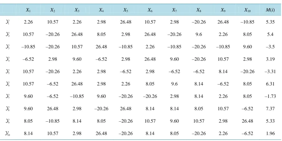
It is necessary to have an example for illustrating the proposed formula to calculate sample size without pre-defined error. Given 10-element sample  = {X1 = 8.05, X2 = 9.60, X3 = 2.98, X4 = –20.26, X5 = –6.52, X6 = –10.85, X7 = 8.14, X8 = 26.48, X9 = 10.57, X10 = 2.26}, we will estimate the optimal size of the next sample

based on . Suppose there are 10 iteration times (m = 10), we have 10 new sample i (s) is sampled

ran-domly from  with replacement. Table 1 shows such 10 new sample i (s) and their means M(i) (s).

The sample variance Δ2

of sample means M(i) (s) is:

( )

( )

(

)

2

10 10

1 1

2

1 10

16.78 10 1

i= M i j=M i

 ₋ 

 

 

∆ = ≈

−

∑

∑

The mean X of sample  is:

10

1

1

3.04 10 j i

X X

=

=

∑

≈

The sample variance s2 of sample  is:

(

)

10

2 2

1

1

169.79 10 1i i

s X X

=

= − =

−

∑

Given the confident level 95% (α = 0.05), it is easy to calculate the optimal sample size as follows:

( )

2

₍

₎

2

(

)

₂

2 2

10 169.79

1.96 43

1 Δ 9 16.78

m s n Z

m

α

= ≈ − ≈

−

[image:4.595.88.539.492.718.2]

According to results from many experiments, if the origin sample (previous sample ) conforms normal distribution, the optimal sample size is 4 - 5 times larger than the size of such origin sample so that it is possible to gain better experiment (testing, analysis, estimation, etc.) because the origin sample that conforms normality is itself good sample. We can implement the proposed formula of sample size choice by R language [3] so that it is convenient to do many experiments on such formula. Following is R language code for implementing the proposed formula.

Table 1. Ten new samples and their means.

X1 X2 X3 X4 X5 X6 X7 X8 X9 X10 M(i)

1

 2.26 10.57 2.26 2.98 26.48 10.57 2.98 –20.26 26.48 –10.85 5.35

2

 10.57 –20.26 26.48 8.05 2.98 26.48 –20.26 9.6 2.26 8.05 5.4

3

 –10.85 –20.26 10.57 26.48 –10.85 2.26 –10.85 –20.26 –10.85 9.60 –3.5

4

 –6.52 2.98 9.60 –6.52 2.98 26.48 9.60 –20.26 10.57 2.98 3.19

5

 10.57 –20.26 2.26 2.98 –6.52 2.98 –6.52 –6.52 8.14 –20.26 –3.31

6

 10.57 –6.52 26.48 2.98 2.26 8.05 9.6 8.14 –6.52 8.05 6.31

7

 9.60 –6.52 –10.85 9.60 –20.26 –20.26 2.98 8.14 2.26 8.05 –1.73

8

 9.60 26.48 2.98 –20.26 26.48 8.14 8.14 8.05 10.57 –6.52 7.37

9

 8.05 –10.85 8.14 8.05 –20.26 10.57 9.60 10.57 2.98 26.48 5.33

10

3. Conclusions

I invent this method when discussing with the co-author Dr. Hang Ho about choice of sample size. At that time, I make the simile that the ideology of this method is similar to the problem “hen and egg”. Regardless that hen exists before or egg exists before, you feed hen to lay new egg and incubate such egg to hatch new hen. There-fore, given an available random sample is used to estimate the sample size and such sample size is applied to collect new random sample; after that new sample size is estimated based on the new random sample and so on. Now, we analyze the formula for estimating sample size:

( )

₍

₎

2

2

2 2

1 Δ

m s n Z

m

α

=

−

The variance s2 in numerator expresses the coherent variation of data and the value Δ2 in denominator speci-fies the variation of disturbed data (data is disturbed for many times). It means that Δ2 specifies the variation of change (or variation of variation). The smaller the value Δ2 is, the more precise the variance s2 is and so the sample size is much proportional to s2. In other words, the small Δ2 makes an increase in sample size. Ratio

1

m m−

approaches 1 when m approaches +∞ and so, the larger the number of iterations is, the more precise the sample

size is. If m is small, the sample size tendentiously increases, but the balance is established because Δ2 will in-crease if m is small, and as known the large Δ2 makes decrease in sample size. But why the small m makes an increase in Δ2

and otherwise? As known the number of iterations m specifies the variation of disturbed data. The larger the number m is, the much more the data is disturbed and so it is easier for the tendency that data is re-verted in equilibrium, which causes the decrease in Δ2

. In other words, the small m makes increase in Δ2.

References

[1] Montgomery, D.C. and Runger, G.C. (2003) Applied Statistics and Probability for Engineers. 3rd Edition, John Wiley & Son, Inc.,Hoboken.

[2] Walpole, R.E., Myers, R.H., Myers, S.L. and Ye, K. (2007) Probability & Statistics for Engineers & Scientists. 9th Edition, Pearson Education, Inc.