Planning of the Operating Points in Desalination Plants based on Energy Optimization

Planning of the Operating Points in Desalination Plants

based on Energy Optimization

Najoua Zarai

University of Sfax CMERP-ENIS, Sfax

Tunisia

Fernando Tadeo

University of Valladolid

47005 Valladolid Spain

Maher Chaabene

University of Sfax CMERP-ENIS, Sfax

Tunisia

ABSTRACT

A methodology is developed for the optimization of the operation of Reverse Osmosis (RO) desalination process. Thus, a computer model of the process is first presented, that comprises two sub models, the first for the solution diffusion process, and the second for the effects of membrane fouling. The optimal operation problem is then stated and transformed into a mathematical optimization problem, based on the minimization of the Specific Energy Consumption (SEC): a computer-based approach is then proposed, to periodically calculate a combination of the pressure difference across the membrane, and the feed water flow rates, that minimizes the SEC, and always fulfils given operational constraints. It is shown that this mathematical problem can be transformed into a standard nonlinear optimization problem, which can be solved using off-the-self software. Application of the methodology is demonstrated on the simulation of a real RO desalination plant, which demonstrates how the proposed approach makes possible to adapt the operation to variations in the plant conditions.

General Terms

Control Systems, Optimization

Keywords

Reverse Osmosis; Energy Consumption; Desalination; Process Control.

INTRODUCTION

A computer based approach is proposed in this paper, to obtain, during operation, the most adequate working point of a Reverse Osmosis (RO) process, and demonstrated on a simulated RO plant. This approach is based on the optimization of the total relative cost of the water produced in 24 hours, taking into account the expected variations of the membranes parameters.

Optimization tools have already been applied to improve RO plants performance, for multistage RO systems [1] and hybrid desalination processes [2]. The application of these techniques has already provided improved designs, efficiencies and operational safety. For example, in [3], an optimization framework was developed to maximize the recovery ratio, or a profit function, using different energy recovery devices subject to general constraints using an efficient successive quadratic programming (SQP) based method. The effects of the arrangement of membrane modules has also been studied in [4], where the operating pressure and the feed flow rate were optimized and demonstrated on a simulated brackish water RO desalination plant. In [5] a systematic methodology for the optimal design of RO desalination system was presented, that considered membrane module cleaning and replacing. A multi-objective optimization using GA was studied for desalination of brackish and sea water using spiral wound or tubular modules in [6]. Recently, optimization has

been used to schedule cleanings, replacement and rotations of membranes within RO plants [7].

All these previous works concentrated on the off-line optimization of the process: i.e., the optimization is carried out independently of the on-line measurements of the process. However, RO plants are known to be time-varying process, as some of their parameters (such as the membrane permeability) change with time in a manner difficult to predict before the operation of plant. Thus, the present paper proposes an optimization technique specific for the operation of RO plants, to select the most adequate operation variables at each time, that minimizes the relative water costs, using available measurements to predict the variations of the plant parameters. For this, some simple models are used to predict the water produced and the energy required, taking into account the expected fouling of the membranes and the cleaning times. The application of the proposed technique to a simulation 5000m3/day RO plant shows that it is possible to reduce the total relative energy cost.

2. MODELLING OF THE SPECIFIC

ENERGY CONSUMPTION OF RO

PLANTS

The energy cost associated with RO desalination is presented in the present analysis as the Specific Energy Consumption (SEC), which is defined as the electrical energy needed to produce a cubic meter of permeate. To simplify the presentation of the approach, the required electrical energy is assumed to be the pump work at the high pressure pump (denoted H.P. pump in Figure 1, that presents a typical RO plant); of course, additional terms can be easily considered by adding them to the optimization [8].

Accordingly, as the one shown in Figure 1 is considered here to be given by

.

pump p

W

SEC

Q



(1)

where

p

Q

is the permeate flow rate and

.

pump

W

is the rate of work done by the pump:

.

f pump

pump

P Q

W



 



(2)

0

f

P

P

P

 



(3)

The pump efficiency



pump

(

Q

p

,



P

)

can be pre-determined from the pump characteristic curve, and estimated from online-measurements. For simplicity, this is assumed here to be constant during the considered time-scale and range of parameters, but it variations can be easily accommodated in the proposed approach. Thus, we just consider the “normalized” SEC given by:

m pump

SEC







SEC

(4)

2.1

Solution Diffusion Model

The model used for estimating the total water costs is based on two submodels: one for the solution and diffusion at membrane level, and the other for the effect of fouling. The first one is now presented.

In the solution-diffusion model [9], the solute and the solvent are assumed to dissolve in the homogeneous non porous surface layer of the membrane and then are transported by diffusion under the chemical potential gradient in an uncoupled manner. The solvent (water) flux Jw is defined as

the volume of water passing through a unit area of the membrane. The water flux Jw, and the solute flux Jsaccording

to solute diffusion transport mechanism are given by [9]:

(

)

p

w

Q

J

a

P

S



    

(4)

(

)

s wall p

J



b C



C

(5)





is the osmotic pressure difference of solute across the membrane,

C

_wall is the solute concentration at the membrane surface,

C

_pis the permeate side solute concentration and Constants a and b are the solvent (membrane) and the solute (salt) permeability coefficients, respectively. The solute concentration at the membrane surface is usually greater than that in the bulk solution due to polarization effects. As water flows through the membrane and salts are rejected by the membrane, a boundary layer with a higher salt concentration is formed near the membrane surface. This increase in salt concentration at membrane surface is called concentration polarization and leads to serious problems during membrane operation as it increases the overall resistance to solvent flux. In the presence of concentration polarization, the steady-state water flow rate Jw is given by:

ln(

wall p

)

w s

b p

C

C

J

k

C

C







(6)

Where

C

_b is the feed side bulk solute concentration. Thus,

exp(

)

(

(

) exp(

))

exp(

)

w b

s w

w b

w s

w

s

J

bC

k

J

J

a

P b C

J

k

J

b

k



  





(7)

exp(

)

b p

w w

s

bC

C

J

b

J

k







(8)

The osmotic coefficient

b

_can be estimated using:

( )

b C

C







(9)

Where C is the concentration of all constituents in the solution, (in kg/m3_{) and  is the osmotic pressure (in bars).}

Equation 4 is an implicit nonlinear algebraic equation that can be solved numerically by the secant method to give Jw for a

set of values of

C

_b, T, a, b,

k

_s,

b

_ and ΔP. The value of

p

C

can then be evaluated using Eq. 5. Also, as p

w

Q

J

S



,

Equations 4 and 5 become:

exp(

)

(

(

) exp(

))

exp(

)

p b

p s

p b

p p _s

s

Q

bC

Q

Sk

Q

aS

P b C

Q

Q

Sk

b

S

Sk





 





(11)

exp(

)

b p

p p

s

bC

C

Q

Q

b

S

Sk







(12)

where S is the active area of the membrane (m2).

2.2

Mass Transfer Coefficients

The mass transfer coefficient can be expressed in an empirical Sherwood relationship taking into account the flow conditions (expressed in the Reynolds number, Re), the nature of the feed solution (expressed by the Schmidt number, Sc) and the geometry of the membrane system [10].

The mass balance is represented by the following equation [11] :

f f p p b b

Q C



Q C



Q C

(13)

whereas the flow balance is given by the following equation;

f p b

Q



Q



Q

(14)

which gives

b f p

Q



Q



Q

(15)

(

)

f f p p b f p

Q C



Q C



C Q



Q

(16)

Using Equation 12, this gives the following relation, that will be used as a constraint in the optimization:

(

)

(1

)

0

exp(

)

b f f b b p

p p

s

bC

Q C

C

C Q

Q

Q

b

S

Sk











(17)

2.3

Modelling of Membrane Fouling

The relation of the water flow rate Jw across the membrane

with the pressure and concentration gradients is assumed to be given by Equation 4. Similarly, the flow of salt across a section of the RO membrane, Js, is given by Equation 5. The

cleaning regimen is assumed to be based on flushing membrane modules by recirculating the cleaning solution at high speed through the module. The water permeability and salt permeability constants are assumed to depend on temperature and fouling, with membrane fouling modeled as an exponential decay of the water permeability over time, with incomplete recovery [12],[13],[14]:

0

0 t

exp

T

T

T

a

A A

a

T









_

_





(18)

0

0 t

exp

T

T

T

b

B B

b

T









_

_

where

A

₀and

B

₀are the membrane coefficients just after cleaning, at the reference temperature

_T

₀



₂₉₁



_K

;

a

_T and

T

b

are dimensionless empirical constants;

A

_t and

B

_t are empirical coefficients, corresponding to membrane fouling (affected by aging and scaling):

1 10

exp(

)

t

t

A







(20) 1 20 exp( ) t t

B  

 (21) Thus, 0 1 0 10

exp(

) exp

T

T

T

t

a

A

a

T











_

_







(22)

0 1

0

20

exp(

t

) exp

_T

T

T

b

B

b

T











_

_







(23)

where t1 is the time duration since the last cleaning;



₁₀and 20



are membrane performance decay constants.

3.

Transformation into a computer

optimization problem

The present study aims to optimize the performance of an existing RO desalination system by computing the operating pressure difference across membrane (



P

), that minimizes the Specific Energy Consumption (SEC), predicted using the model developed in Section 2. This optimization is constrained by some operating constraints, on the permeate concentration, the brine concentration, and the feed water pressure and flow rate. In order to take into account the time-varying characteristics of the desalination process, a

methodology borrowed from Predictive Control

(Maciejowski, 2001) will be used: the operation variables (Pressure

P

_f and Flow

Q

_f of the pretreated flow) will be estimated not only at the current time, but also during a “prediction horizon” (assumed here to be 24 hours). Using this technique, it is possible to include the effect of the operating parameters variations on the aggregated SEC value during the “prediction horizon” (Thus, the energy used can be distributed to use it when most water can be used). Note that this approach makes also possible to consider variations in the costs of energy, but this is left as further work. Thus, for a given RO system layout (number of channels, membrane area, etc.), the single objective function

Z

to be minimized is:

24 1

( )

( )

( )

f f k p

Q k

P k

Z

Q k









(24)

where k goes from 1 (current time) to 24 (1 day ahead): of course, although it is assumed here that the operating point is adapted every hour; other values can be trivially accommodated in the proposed technique.

The constraints are then given as:

( ) ( )

( ) ( )

( ) ( )

( )

min

( )

max

min

( )

max

min

( )

max

f f

f f

p p

p desired

P k f P k

Q k f Q k

Q k p Q k

C k

C

P k

Q k

Q k















This optimization can be carried out on-line, every hour, using off-the-self software, as shown in next section.

24 1 ( ) ( ) min ( ) exp( ) ( )

( ( ) ( ) exp( ))

( ) ( )

exp( )

(1, 2,..., 24)

(1, 2,..., 24)

( )

exp( )

( )

( ) ( ( ) ( ) exp( ))

( ) ( ) exp( ) ( ) ( f f p k b p s f b

p p s

s f f p b p s

p f b

p p s

s f f p

Q k P k

Q k bC

Q k Sk

aS P k b C

Q k Q k Sk

b S Sk P Q Q k bC Q k Sk

Q k aS P k b C

Q k Q k Sk

b

S Sk

Q k C Q k

           



( ) ( ) ( ) ( ) ( ) ( ) ) ( ) ( ( ) ( )) ( ) ( ) ( ) exp( ) ( )

min ( ) max

min ( ) max

min ( ) max

f f

f f

p p

p b f p

b p

p p

s p desired

P k f P k

Q k f Q k

Q k p Q k

C k C Q k Q k

bC C k

Q k Q k

b

S Sk

C k C

P k Q k Q k            

3.1 Transformation into a standard optimization problem

In order to transform the proposed optimization problem into a nonlinear optimization problem that can be used in a computer using commercially available software, we define the following vector of unknown variables:

   

     

     

 

1 1 1 2 1 24 2 1 2 2 2 24 3 1 3 2 3 24

x x x x x x x x x x _

where

x i

₁

 

denotes

P i

_f

 

,

x i

₂

 

denotesQ i_f

 

, and

x i

₃

 

denotes _{Q ip}

 

.

Using this variables, the proposed optimization problem can then be written in a more compact and general form as

   

 

1 2 1 3 1

min

n i n x i

x i x i

x i

 





(25) subject to

 

 

 

 

 

 

 

 

_{ }

_{ }

 

 

3 3 3 1 3 3 2 3 3 3 3 3 exp( )

( ( ) exp( )) 0

exp( )

( ) (1 ) 0

exp( ) 0.35 exp( ) b s b s s b f b b

s b s x i bC x i Sk

x i aS x i b C

x i x i Sk

b

S Sk

bC

x i C C C x i

x i x i

b

S Sk

bC

x i x i

This is a standard nonlinear optimization problem that can be solved with any of the available methods, for example using Matlab or GAMS.

In the above optimization the permeability parameters a[i] and b[i] are given: they can be pre-calculated using a prediction model based on the state of the plant: cleaning times and the estimated rate of fouling. For example, the following model can be used, that corresponds to Equations 18 to 23, with cleaning at i=0:

 

 

0 0

10

0 0

20

1...24

exp(

) exp

exp(

) exp

T

T

i

T

T

i

a i

A

a

T

T

T

i

b i

B

b

T













_

_

















_

_







This can be easily incorporated into the optimization problem in (24). If necessary, more complex fouling models can be used.

4.

RESULTS AND DISCUSSION

In order to validate the techniques, a benchmark RO plant (extracted from the literature [9]) was used. Some results are now presented and discussed.

Description of the RO system

In [9] an 5000 m3_{/day RO Plant with the structure shown in}

[image:4.595.323.559.86.436.2] [image:4.595.57.200.181.238.2]

Figure 1 was studied. The nominal parameters, used for modeling and simulation of the process, are condensed in Table 1.

Table 1: Simulation parameters

Parameters Values

Cb Concentration of the brine (kg/m3) 44

bπ Osmotic coefficient (bar.m3/kg) -

S Area of the membrane (m2) 2090

A0 Membrane coefficients just after

cleaning

5.5 10-7

B0 Membrane coefficients just after

cleaning

1.8 10-5

aT Dimensionless empirical constant 3

bT Dimensionless empirical constant 3.08

T Temperature of the membrane (°C) 28

T0 Reference Temperature (°C) 25

Γ10 Membrane performance decay

constant (h)

328

Γ20 Membrane performance decay

constant (h)

650

3.2 Validation

Extensive tests were carried out to check the proposed approach on the target plant. The osmotic pressure was estimated to be:

2 5 3 7 4

0.7949

C

0.0021

C

7.0 10

C

6.0 10

C



_

_

_

_



_

_



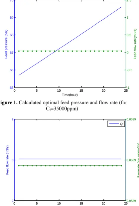
As an example, the results of one of these experiments (when Cf=35000ppm) are presented: Figure 1 presents the proposed

Feed pressure and Feed flow rate for the system discussed in section 4.1, assuming cleaning of the membrane at time 0. It can be seen that the optimization effectively evolves the operating point, maintaining the pump Pressure and decreasing linearly the flowrate, which creates the variations in production shown in Figure 2. The use of energy is presented in Figure 3).

0 5 10 15 20 25

65 66 67 68 69 70

F

e

e

d

p

re

s

s

u

re

(

b

a

r)

Time(hour)

0 5 10 15 20 25-1

-0.5 0 0.5 1 1.5

F

e

e

d

f

lo

w

r

a

te

(m

3

/s

)

Figure 1. Calculated optimal feed pressure and flow rate (for Cf=35000ppm)

0 5 10 15 20 25

-2 0 2

F

e

e

d

f

lo

w

r

a

te

(

m

3

/s

)

Time(hour)

0 5 10 15 20 250.0539

0.0539 0.0539

P

e

rm

e

a

te

f

lo

w

r

a

te

(m

3

/s

)

Qf

Figure 2. Calculated optimal feed and permeate flow rates

0 5 10 15 20 25

49.5 50 50.5 51 51.5 52 52.5 53

Time(hour)

E

n

e

rg

y

c

o

n

s

u

m

e

d

(

b

a

[image:4.595.48.288.412.591.2]

r)

Fig 3. Estimated energy consumed by the RO process

3.3 Discussion

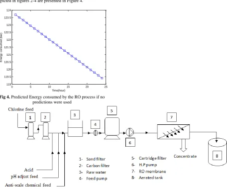
[image:4.595.325.538.475.645.2]

It must be pointed out that with the proposed minimization, which is based on planning the operating points for the next 24 hours, smaller total energy costs are obtained, when compared with the simpler approach of planning the operating point only for the current hour. This is thanks to the fact that the proposed approach distributes the use of energy throughout the whole day (Thus, using slightly more energy when the conditions are predicted to be favourable). This utility of predictions is clear when the available energy changes, but it can be easily seen also when the available energy is not limited, by comparing the optimal value obtained using (25), with the one obtained when no prediction is used: that, is, from the following expression:

   

 

1 2

1 3

min

n_i

x

x i x i

x i





(26)

subject to the equivalent constraints; for example, with the proposed approach the optimal value obtained of the Specific Energy Consumption is presented in Figure 3.

This can be compared with the no-prediction case of eq. (26): the optimal values of the (SEC) for the same experiment depicted in figures 2-4 are presented in Figure 4.

0 5 10 15 20 25

119 119.5 120 120.5 121 121.5 122 122.5 123 123.5 124

Time(hour)

E

n

e

rg

y

c

o

n

s

u

m

e

d

(

b

a

[image:5.595.62.519.309.689.2]

r)

Fig 4. Predicted Energy consumed by the RO process if no predictions were used

5.

CONCLUSIONS

This paper has presented a practical proposal to estimate during operation of a Reverse Osmosis process the most adequate working points in the next 24 hours, through optimization of the total relative cost of the water expected to be produced during the next 24 hours. For this, some simple models are used to predict the water produced and the energy required, taking into account the fouling of the membranes and the cleaning times. The proposed technique has been applied on a simulation of a 5000m3/day RO plant, showing that using the proposed technique it is possible to reduce the total relative energy cost. It must be pointed out that the proposed methodology was developed as the basis of the solution of more complex operation problems. For example, some operation parameters (such as the level of fouling) can be identified online, which makes possible to improve the predictions and thus reduce the total energy costs. Moreover, it can be integrated with prediction models of the available energy and costs [15], in order to reduce the overall operation costs.

Nomenclature

At empirical coefficient

Bt empirical coefficient

bπ osmotic coefficient

Cp concentration of the permeate (kg m3)

Cp,d desired permeate concentration (kg m3) t1 time of the last cleaning (s)

Cwall concentration at the wall membrane (kg m3) t time (s)

d channel height (m) v velocity of feed water (m/h)

dh hydraulic diameter of channel (m)

dSP spacer thickness (m) Δ difference

DAB Mass diffusivity of salt through water (m2/h) ε void fraction (bulk porosity)

Jw volumetric flux of water (m/h) µ dynamic viscosity (Pa.s)

Js mass flux of salt (kg/m2.h) π osmotic pressure (bar)

ks mass transfer coefficient (m/h) ρ density of sea water (kg/m3)

P pressure (bar) η efficiency

Qf feed water volumetric flow rate (m3/h) ν Kinematic viscosity (m2/h)

Qw permeate volumetric flow rate (m3/h)

Re Reynolds number Subscripts

S Sc

area of the membrane (m2₎

Schmidt number

b w

brine water

Sh Sherwood number f feed

T temperature (°C) p permeate

6.

ACKNOWLEDGMENTS

This work was partially funded by MiCInn project DPI2010-21589-c05.

7.

REFERENCES

[1] Marcovecchio, M.C., Aguirre, P.A., and Scenna, N.J., Global Optimal Design of Reverse Osmosis Networks for Seawater Desalination: Modeling and Algorithm, Desalination, Vol. 184, 2005, pp. 259-271.

[2] Helal, A.M., El-Nashar, A.M., Katheeri, E., and Al-Malek, S., Optimal Design of Hybrid RO/MSF Desalination Plants - Part II: Results and Discussion, Desalination, Vol. 160, 2004, pp. 13-27.

[3] Villafafila, A., and Mujtabab, I.M., Fresh Water by Reverse Osmosis Based Desalination: Simulation and Optimisation, Desalination, Vol. 155, 2003, pp. l-13.

[4] Abbas, A., Simulation and Optimization of an Industrial Reverse Osmosis Water Desalination Plant, Proceedings of International Mechanical Engineering Conference, December 5-8, 2004, Kuwait, IMEC04-2056.

[5] Lu, Y.Y., Hu, Y.D., Xu, D.M., and Wu, L.Y., Optimum Design of Reverse Osmosis Seawater Desalination System Considering Membrane Cleaning and Replacing, Journal of Membrane Science, Vol. 282, 2006, pp. 7-13.

[6] Guria, C., Bhattacharya, P.K., and Gupta, S.K., Multi-Objective Optimization of Reverse Osmosis Desalination Units using Different Adaptations of the Non-Dominated Sorting Genetic Algorithm (NSGA), Computers and Chemical Engineering, Vol. 29, 2005, pp. 1977-1995.

[7] Palacin, L.G., Tadeo, F., Prada, C. de, and Salazar, J., Scheduling of the Membrane Module Rotation in RO Desalination Plants, Desalination and Water Treatment, 2012 (In press).

[8] Li, M., Minimization of Energy in Reverse Osmosis Water Desalination Using Constrained Nonlinear Optimization, Ind. Eng. Chem. Res, 2010.

[9] Berge. D, Helmy, G., Ibrahim, K., Magdy, A.R, Optimization of Reverse Osmosis Desalination system using Genetic Algorithms Technique, 12th International Water Technology Conference, Alexandria, Egypt, 2008.

[10]Taniguchi, M., Kurihara, M., and Kimura, S., Behavior of a Reverse Osmosis Plant Adopting a Brine Conversion Two-Stage Process and its Computer Simulation, Journal of Membrane Science, Vol. 183, 2001, pp. 249-257.

[11]Kamal, M., Sassi, I., Mujtaba, M., Simulation and

Optimization of Full Scale Reverse Osmosis

Desalination Plant, 20th European Symposium on Computer Aided Process Engeneering,2010.

[12]Palacin, L. G., F. Tadeo, H. Elfil, C. de Prada, J. Salazar, New dynamic library of reverse osmosis plants with fault simulation, Desalination and Water Treatment, DWT 7281, Volume 25, 2011, 127-132.

[13]L. G. Palacin, F. Tadeo, C. de Prada, H. Elfil, J. Salazar, Operation of desalination plants using hybrid control, Desalination and Water Treatment, DWT 7280, Volume 25, 2011, 119-126.

[14]Luis Palacin, Fernando Tadeo, Cesar de Prada, Desalination In Remote Areas: A Prediction-Based Approach, IDA World Congress 2011, Perth, Australia, 2011.