Mining Time Variant Frequent Pattern using PPM and PWM: A Comparison

(1)

Mining Time Variant Frequent Pattern using PPM and

PWM: A Comparison

P. A. Shirsath

M.Tech (CSE)

Lord Krishna College of Technology, Indore

Vijay Kumar Verma

Assistant Professor M. Tech (CSE) Lord Krishna College of Technology, Indore

ABSTRACT

The process of exploring and analyzing data from different perspective, using automatic or semiautomatic techniques is called Data mining. Data mining extracts knowledge or useful information and discovers correlations or meaningful patterns and rules from large databases [1, 2]. Using these patterns and rules it is possible for business enterprises to identify new and unexpected trends, subtle relations in the data and use them to increase revenue and cut cost. In this paper we proposed a comparative study over Progressive Partition Miner (PPM) and Progressive Weighted miner (PWM).

Keywords

Progressive, Partition, Miner, Weighted, Comparative

1. INTRODUCTION

The traditional data mining techniques not have ability to analyse variation of data over time and treat them as ordinary data. Temporal datasets includes stock market data, manufacturing or production data, maintenance data, web mining and point-of-sale records. Temporal data mining means mining or discovering knowledge and patterns from temporal databases. Temporal data mining is an extension of data mining with ability to include time attribute analysis. Due to the significance and complexity of the time attribute, a lot of different kinds of patterns are of interest [3, 5].

Two time aspects are included in temporal databases namely, valid time and transaction time. The time period during which a fact is true with respect to the real world is considered as valid time and the time period during which a fact is stored in the database is called transaction time. According to these two time aspects temporal databases allow the division of three different forms [4, 25]. They are

a. A historical database stores data with respect to valid time.

b. A rollback database stores data with respect to transaction time.

c. A bitemporal database stores data with respect to both valid and transaction time, that is, they store the history of data with respect to valid time and transaction time.

2. TEMPORAL DATA MINING TASKS

A main question is how to apply traditional data mining techniques on a temporal database. Temporal data mining may involve the following areas of investigation. Temporal data mining tasks includes:

i. Temporal association rules

ii. Temporal data classification and comparison iii. Temporal pattern analysis

iv. Temporal clustering analysis

v. Temporal prediction and trend analysis vi. Temporal classification [6]

3. RELATED WORK

A temporal association rule is defined as the frequency of an itemset over a time period T and is the number of transactions in which it occurs divided by total number of transaction over a time period. To solve the problem on handling time-series by including time expression into association rules temporal association rule mining has been introduced. Temporal association rule mining is first introduced by Wang, Yang and Muntz in years 1999-2001.Temporal association rule mining is introduced together with the introduction of the TAR (Temporal Association Rule) algorithm. With the help of Temporal association we can finds the valuable relationship among the different item sets, in temporal database. There are several types of temporal association rules defined by various researcher e such as inter transaction rules, episode rules, trend dependencies, sequence association rules [6, 7, 8].

Roddick and Spiliopoulou (2002) have presented a comprehensive overview of techniques for the mining of temporal data using three dimensions: data type, mining operations and type of timing information (ordering).

Winarko and Roddick, 2005 proposed a non Apriori-based technique that avoids multiple database scans, this methods not only avoid multiple data scan but efficiently mine arrangements and rules in a temporal database. The main drawback of this method is that it do not consider any constraints for the temporal relations and do not examine any measures for their rules other than the traditional confidence [9].

Tansel and Imberman (2007) proposed a method where association rules were extracted for consecutive time intervals with different time granularities. They proposed a simple operation that extracts portions of a temporal relation was used during mining process and was combined with the first step of discovering association rules. Using this approach, the process of knowledge discovery can observe the changes and variation in the association rules over the time period when these rules are valid [10, 11].

Gharib et al. (2010) proposed a method for generating temporal association rules to solve the problem of handling time series by including time expressions into association rules. To solve this they extended an incremental algorithm to maintain the temporal association rules in a transaction database, at the same time maintains the benefits from the results of earlier mining to derive the final mining output [7, 12, 14].

(2)

Volume 77– No.15, September 2013

infrequent 2-itemsets. PPM efficiently reduction extra scanning process. PPM works efficiently with temporal datasets. However, the limitation of this technique is its ability to deal with problems of incremental mining [7, 9, 17].

Cheng. Y. Chang et al Segment Progressive Filter (SPF) was introduced after PPM. SPF is based on the Segmentation and progressive filtering. It was introduced. SPF first divide the database into certain imposed time granularity. It further segments the database based on their common starting and ending times. For each part of the database it finds the 2-candidate item set with appropriate filtering threshold. After generating all candidates it generates the sub-candidate and counts for the value of support. Temporal databases are continuously updated or appended [13, 16].

[image:2.595.364.486.76.256.2]

Ru Miao et al presented the idea of Apriori-extended mining periodic temporal association rules (MPTAR). MPTAR solved this problem, by considering the exhibition period of individu.al item. MPTAR is also a two-step periodic rule mining method. The first step is mining the trend of continues attribute through cycle curve and the second step is calculating the period of the attribute. MPTAR did not define the cumulative threshold, and it is short of embracing upcoming transaction entries in the association rule mining [15, 18, 25].

4. BASIC CONCEPTS

Temporal association rule adds time constraint (it can be time point or time range) on association rule. A transaction with time information can be described as: {TID, I1, I2 …In, Ts, Te}. TID is the ID for each transaction; n-itemsets means there are n items in the itemset; Ts and Te represent the start and the end of valid time respectively (or the start and the end of transaction). Valid time means the event occurring time, while transaction time the database time. Ts may equal Te, such as sale records in the supermarket (the transaction occurs at one moment). According to the definition of strong association rule “association rule strictly satisfies minimum support threshold and minimum confidence threshold”, we can give the definition of strong temporal association rule [6, 19, 10].

Let min_s and min_c represent minimum support threshold and minimum confidence threshold respectively, if and only if during [ts, te], support ≥ min_s, confidence ≥ min_c, rule X→Y is a temporal association rule, which could be described as X→Y (support, confidence, [ts, te]).

5. TEMPORAL ASSOCIATION RULE

MINING METHODOLOGY

Temporal data mining has become a core technical data processing technique to deal with changing data. Temporal Association Rules (TAR) is an interesting extension to association rules by including a temporal dimension. No matter what kinds of tools or algorithms you select, strong temporal association rule mining can be divided into 3 steps.

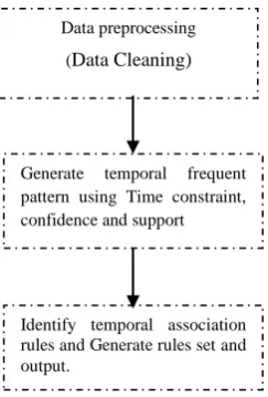
Fig 1: Working process of mining temporal association rule

First step is Data pre-processing. Data pre-processing performs several steps to improve the quality of the input dataset. This is an important step of data mining. Data pre-processing include removal of unwanted or irrelevant data, integration of databases and data exchange and data reduction. By processing, we can get high quality data mining objects.

Seconds step uses time constraints on the two parameters support and confidence to generate temporal frequent itemsets. All the generated temporal frequent itemsets have the support no less that min support.

Third step generate association rules with frequent itemsets. Here the association rules are temporal ones. Since it is different to generate association rules without time, because it adds time information on frequent itemsets.

6. PROGRESSIVE PARTITION MINER

(PPM)

Basic steps used in PPM are [3, 24]

A. It Stores candidate 2-itemsets from previous mining process with their support counts using time.

B. It employs the skeleton of the incremental procedure of the Sliding-Window Filtering algorithm.

Working of PPM is shown by following flowchart Data preprocessing

(Data Cleaning)

Generate temporal frequent pattern using Time constraint, confidence and support

Identify temporal association rules and Generate rules set and output.

2nd scan 1st scan

Partition database according to exhibition period

Generate frequent candidate 2-itemset for first partition by considering minimum support

Generate 2 itemsets for next partition and use generated frequent itemsets to find frequent itemsets in both partitions

(3)

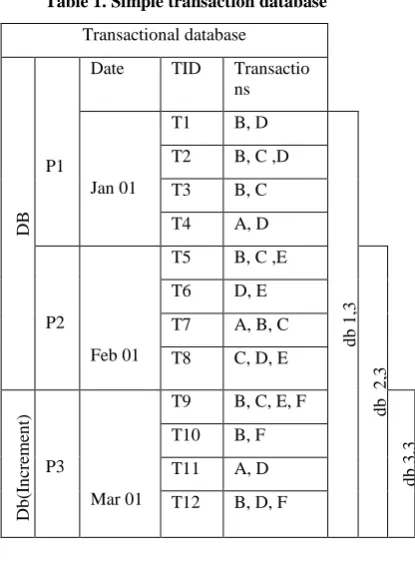
Consider a simple transaction database

Table 1. Simple transaction database

Transactional database

DB

DB (Orig

in

al

d

atab

ase

)

P1

Date TID Transactio ns

Jan 01

T1 B, D

d

b

1

,3

T2 B, C ,D

T3 B, C

T4 A, D

P2

Feb 01

T5 B, C ,E

db

2

,3

T6 D, E

T7 A, B, C

T8 C, D, E

Db

(In

cre

m

en

t)

P3

Mar 01

T9 B, C, E, F

d

b

3

,3

T10 B, F

T11 A, D

T12 B, D, F

[image:3.595.323.506.57.746.2]

i. Let minimum is support 30% now generate two item set for P1

Table 2. Candidate item set for p1

P1

C2 Start Count

AD 1 1

BC 1 2

BD 1 2

CD 1 1

ii. Now check candidate item set for P1 minimum support 4*0.3=1.2

Table 3. Frequent item set for P1

P1

C2 Start Count

BC 1 2

BD 1 2

[image:3.595.370.480.65.423.2]

iii. Generate two item set for P1+P2

Table 4. Candidate item set for P1+P2

P2

C2 Start Count

AB 2 1

AC 2 1

BC 2 2

BE 2 1

CD 2 1

CE 2 2

DE 2 2

+

P1

C2 Start Count

BC 1 2

BD 1 2

P1+P2

C2 Start Count

AB 2 1

AC 2 1

BC 1 4

BD 1 2

BE 2 1

CD 2 1

CE 2 2

DE 2 2

[image:3.595.68.501.80.797.2]

iv. Support count for P1+P2= (4+4)*.03 = 2.4

Table 5. Frequent item set for P1+P2

P1+P2

C2 Start Count

BC 1 4

CE 2 2

DE 2 2

v. Now generate candidate item set for P3+P2+P1

Table 6. Candidate item set for P1+P2+P3

P3

C2 Start Count

AD 3 1

BC 3 1

BD 3 1

BE 3 1

BF 3 3

CE 3 1

CF 3 1

DF 3 1

[image:3.595.60.269.82.811.2] [image:3.595.61.269.91.373.2]

(4)

P1+P2

C2 Start Count

BC 1 4

CE 2 2

DE 2 2

P1+P2+P3

C2 Start Count

AD 3 1

BC 1 5

BD 3 1

BE 3 1

BF 3 3

CE 2 3

CF 3 1

DE 2 2

DF 3 1

EF 3 1

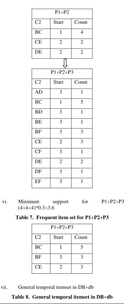
[image:4.595.59.271.55.571.2]

vi. Minimum support for P1+P2+P3= (4+4+4)*0.3=3.6

Table 7. Frequent item set for P1+P2+P3

P1+P2+P3

C2 Start Count

BC 1 5

BF 3 3

CE 2 3

vii. General temporal itemset in DB+db

Table 8. General temporal itemset in DB+db

Itemset Start End Start End TI

B C

BC 1 3 1 3 BC1,3

B F

BF 1 3 3 3 BF3,3

C E

CE 1 3 2 3 CE 2,3

[image:4.595.366.481.101.246.2]

viii. General sub temporal item set in DB+db

Table 9. General subtemporal itemset in DB+db

TI SI

BC1,3 B1,3

C 1,3

BF3,3 B 3,3

F 3,3

CE 2,3 C 2,3

E 2,3

7. PROBLEM STATEMENT

In our opinion, the existing model of the constraint based association rule mining is not able to efficiently handle the time-variant database due to two fundamental problems

1. Lack of consideration of the exhibition period of each individual transaction

2. Lack of an intelligent support counting basis for each item [20, 21].

8. PROGRESSIVE WEIGHTED MINER

(PWM)

In Partition Weighted Miner the importance of each transaction period is first reflected by a proper Weight assigned by the user. Then time-variant database in light of weight periods of transactions and performs weight mining. Explicitly, Progressive Weighted Miner explores the mining of weighted association rules, denoted by (X → Y) w, which is produced by two newly defined concepts of weight support and weight confidence in light of the corresponding weight in individual transactions [22, 23].

Basically, an association rule X → Y is termed to be a frequent weight association rule (X → Y )w if and only if its weight support is larger than minimum support required, i.e., supp_w (X → Y) > min_supp, and the weight confidence conf W (X → Y) is larger than minimum confidence needed, i.e., conf_w (X → Y ) > min_conf. Instead of using the traditional support threshold min_sT = {d|D|×min_sup} as a minimum support threshold for each item, a weight minimum support, denoted by min_Sw = {Σ|Pi|×W (Pi)} ×min_supp, is employed for the mining of weight association rules, where |Pi| and W (Pi) represent the amount of partial transactions and their corresponding weight values by a weight function W (·) in the weight period Pi of the database D.

Let NPi(X) be the number of transactions in partition Pi that contain itemset X. The support value of an itemset X can then be formulated as Sw(X) = ΣNPi(X)×W(Pi). As a result, the weight support ratio of an itemset X is suppw (X) = Sw (X) / [Σ|Pi|×R (Pi)].

(5)

83.3% and (F →B)w with relative weight support suppw (F → B) = 42.8% and confidence conf w (F → B) = 100% [11].

Consider the previous transactional data base candidate set for P1 with minimum weight support.

i. Candidate itemset for p1

Table 10. Candidate item set for P1

[image:5.595.332.508.64.347.2]

ii. Candidate set for P1+P2 with minimum weight support

Table 11. Candidate item set for P1+P2

min_S C(P1+P2)=1.8, min_S C(P2)=1.8

C2 Start NW(X) count

AB 2 1*1=1

AC 2 1*1=1

BC 1 1+2*1=3 *

BD 1 1+0*1=1

BE 2 1*1=1

CD 2 1*1=1

CE 2 1*1=1 *

DE 2 1*1=1 *

[image:5.595.61.252.254.763.2]

iii. Candidate set for P1+P2+P3 with minimum weight support

Table 12. Candidate item set forP1+P2+P3

min_S C(P1+P2+P3)=4.2,

min_S C(P2+P3)=3.6, min_S C(P3)=2.4

C2 Start NW(X) count

AD 3 1*2=2

BC 1 3+1*2=5 *

BD 3 1*2=2

BE 3 1*2=2

BF 3 3*2=6 *

CE 2 2+1*2=2 *

CF 3 1*2=2

DE 2 2+0*2=2

DF 3 1*2=2

EF 3 1*2=2

iv. Final frequent itemset is

Table 13. Frequent item set forP1+P2+P3

P1+P2+P3

C2 Start Count

BC 1 5

BF 3 3

CE 2 3

Finally we can generate same frequent item set which generated by the PWM by using simple weight function.

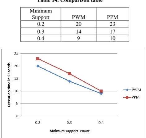
7. EXPERIMENTAL RESULTS

[image:5.595.313.549.507.729.2]

For the experimental analysis, we execute the algorithm PPM and PWM for 25 items with 10,000 transaction .Form the graph it is clear that PWM takes less execution time as compared to PPM but PWM work more efficiently When the new item came for particular time interval otherwise it work same as PPM .One more thing that are consider with the PWM we have to check the one item set of the previous time interval to find new item set for current scanning time interval.

Table 14. Comparison table

Fig 2: Comparison graph min_s R(P1)=0.6

C2 Start NR(X) count

AD 1 1*0.5=0.5

BC 1 2*0.5=1 *

BD 1 2*0.5=1 *

CD 1 1*0.5=0.5

Minimum

Support PWM PPM

0.2 20 23

0.3 14 17

[image:5.595.84.248.693.785.2]

(6)

8. CONCLUSION

PPM focus on successive partition and calculate frequent item set and PWM assign weight to the partition in successive manner if new item are appears important to note that if we adopt single min_supp = 30% by Apriori, then the itemset {BF} will not be large since its occurrence in this transaction database is 3 which is smaller than min_ST = [12×0.3] = 4. However, itemset {BF} appears very frequently in the most recent partition of the database of which the weight is relatively large, thus discovering more desirable information. It can be seen that the algorithm Apriori is not able to discover the information behind the new coming data in the transaction database.

9. REFERENCES

[1] J. Han, M. Kamber, Data mining, Concepts and techniques, Academic Press, 2003.

[2] Arun K. Pujari, Data mining Techniques, University Press (India) Private Limited 2006.

[3] D. Hand, H. Mannila, P. Smyth, Principles of Data Mining, Prentice Hall of India, 2004.

[5] N. Pughazendi, Dr. M. Punithavalli, “Temporal databases and frequent pattern mining techniques”, International Journal of P2P Network Trends and Technology July to Aug Issue 2011

[6] Weiqiang Lin, Mehmet A. Orgun, Graham J. Williams, “An Overview of Temporal Data Mining”, The Australasian Data Mining Workshop.

[7] Mohsin Naqvi, Kashif Hussain, Sohail Asghar, Simon Fong, “Mining Temporal Association Rules with Incremental Standing for Segment Progressive Filter”

[9] Chang-Hung Lee, Cheng-Ru Lin, and Ming-Syan Chen, “On Mining General Temporal Association Rules in a Publication Database”

[10] ZHAI Lianga, TANG Xinming, LI Lina, JIANG Wenliang, “Temporal Association Rule Mining Based On T-Apriori Algorithm And Its Typical Application”

[11] Chang-Hung Lee1, Jian Chih Ou, and Ming-Syan Chen, “Progressive Weighted Miner: An Efficient Method for Time-Constraint Mining”

[12] Anour F.A., Dafa-Alla, Ho Sun Shon, Khalid E.K. Saeed, Minghao Piao, Un-il Yun, Kyung Joo Cheoi and Keun Ho Ryu “IMTAR: Incremental Mining of General Temporal Association Rules”, Journal of Information Processing Systems, Vol.6, No.2, June 2010

[13] Sotiris Kotsiantis, Dimitris Kanellopoulos, “Association Rules Mining: A Recent Overview

GESTS”, International Transactions on Computer Science and Engineering, Vol.32 (1), 2006, pp. 71-82

[14] Litvak Marina, “Temporal Mining Algorithms: Generalization and Performance Improvements”, The research work for this thesis has been carried out at Ben-Gurion University of the Negev under the supervision of Prof. Ehud Gudes November 2004

[15] D.sujatha, Prof. B. Deekshatulu, “Algorithm for mining time varying frequent itemsets”, Journal of theoretical and applied information technology 2005 - 2009.

[16] Tannu Arora1, Rahul Yadav2, “ Improved Association Mining Algorithm for Large Dataset”, IJCEM International Journal of Computational Engineering & Management, Vol. 13, July 2011

[17] Mamta Dhanda, Sonali Guglani, Gaurav Gupta, “Mining Efficient Association Rules Through Apriori Algorithm Using Attributes”, IJCST Vol. 2, Issue 3, September 2011

[18] Chin-Chen Chang , Yu-Chiang Li ,Jung-San Lee, “ An Efficient Algorithm for Incremental Mining of Association Rules”, Proceedings of the 15th International Workshop on Research Issues in Data Engineering: Stream Data Mining and Applications (RIDE-SDMA’05) © 2005 IEEE

[19] N.L. Sarda, N. V. Srinivas, “An Adaptive Algorithm for Incremental Mining of Association Rules”, Authorized licensed use limited to: Indian Institute of Technology Bombay. Downloaded on April 24, 2009 at IEEE Explore.

[20] Sotiris Kotsiantis, Dimitris Kanellopoulos, “Association Rules Mining: A Recent Overview GESTS”, International Transactions on Computer Science and Engineering, Vol.32 (1), 2006, pp. 71-82

[21] Sandhya Rani Jetti, Sujatha D, “Mining Frequent Item Sets from incremental database:A single pass approach”, International Journal of Scientific & Engineering Research, Volume 2, Issue 12, December-2011 1 ISSN 2229-5518

[22] Jyoti Jadhav, Lata Ragha, Vijay Katkar Incremental Frequent Pattern Mining International Journal of Engineering and Advanced Technology (IJEAT) ISSN: 2249 – 8958, Volume-1, Issue-6, August 2012

[23] Ratchadaporn Amornchewin , Worapoj Kreesuradej, “Incremental Association Rule Mining Using Promising Frequent Itemset Algorithm”, 1-4244-0983 2007 IEEE

[24] Sheila A. Abaya “Association Rule Mining based on Apriori Algorithm in Minimizing Candidate Generation”, International Journal of Scientific & Engineering Research Volume 3, Issue 7, July-2012 1 ISSN 2229-5518