An Uncertain Programming Model for Competitive Logistics Distribution Center Location Problem

(1)

http://dx.doi.org/10.4236/ajor.2015.56042

An Uncertain Programming Model for

Competitive Logistics Distribution

Center Location Problem

Bingyu Lan

1

, Jin Peng

2

, Lin Chen

3

1_{College of Mathematics and Sciences, Shanghai Normal University, Shanghai, China} 2_{Institute of Uncertain Systems, Huanggang Normal University, Hubei, China} 3_{Institute of Systems Engineering, Tianjin University, Tianjin, China}

Received 10 October 2015; accepted 24 November 2015; published 27 November 2015

This work is licensed under the Creative Commons Attribution International License (CC BY). http://creativecommons.org/licenses/by/4.0/

Abstract

We employ uncertain programming to investigate the competitive logistics distribution center lo-cation problem in uncertain environment, in which the demands of customers and the setup costs of new distribution centers are uncertain variables. This research was studied with the assump-tion that customers patronize the nearest distribuassump-tion center to satisfy their full demands. Within the framework of uncertainty theory, we construct the expected value model to maximize the ex-pected profit of the new distribution center. In order to seek for the optimal solution, this model can be transformed into its deterministic form by taking advantage of the operational law of un-certain variables. Then we can use mathematical software to obtain the optimal location. In addi-tion, a numerical example is presented to illustrate the effectiveness of the presented model.

Keywords

Competitive Location, Logistics Distribution Center, Uncertain Programming, Uncertainty Theory

1. Introduction

(2)

to distribution system design.

A large part of location problems have been studied in an ideal environment, in which only a unique facility offers services or products in the market. In practice, with the rapid development of economic, the environment is growing more complex. The facility has to compete with other players for more benefits. Thus the research on competitive location problem plays an important role in location theory. Competitive location problem differs from the general location problem because we must consider the competition between the existing facilities and new facilities. The briefly explain of the competitive location problem is that some facilities have been located in the market and the new facility will be located at the optimal place so as to compete with others for their market share.

Because of the importance of competitive location problem, many scholars devoted to the related research of competitive location problem in deterministic environment, that is, all parameters are known in advance and as-sumed to be fixed. Hotelling [3] initially introduced the competitive problem of two companies in the market, which laid the foundation for modern competitive location problem. Subsequently, a lot of scholars also studied this topic and made a progress in competitive location theory. In location space aspect, the competitive location problem was extended to the planar location problem by Drezner [4]. Moreover, it was also applied to the net-work location problem by Hakimi [5]. So Plastria [6] overviewed the papers of competitive location and clari-fied the location spaces into three traditional spatial settings: discrete space, continuous space and the network. In competition feature aspect, except for the simplest static competitive models, the dynamic models were pro-posed to describe the action cycles of competing players. Wong and Yang [7], and Yang and Wong [8] proposed a continuous equilibrium model, respectively. These models solved the competitive location problem with dif-ferent assumptions of customer demands. With considering the future competition which known in the economic literature as Stackelberg equilibrium problem or leader-follower problem, Plastria and Vanhaverbeke [9] pro-posed three models to solve Stackelberg equilibrium problem in discrete space. The game theory was introduced into the competitive location problem by Küçükaydin et al. [10], in which they formulated a bilevel mixed- integer nonlinear programming model to solve the leader-follower problem. Sasaki et al. [11] employed a ge-neric hub arc location model to locate arcs within the framework of Stackelberg. With respect to methodology, various approaches were proposed to obtain the estimate of the market share captured by each competitive facil-ity, such as proximity approach [4], deterministic utility approach [12], cover-based approach [13], and gravity- based approach [14]. For a detailed view of the models of competitive location problem, see Drezner [15] and Plastria [6].

In practical life, there are many indeterminacy factors in competitive location problem. For example, the de-mand of customer for a kind of product is variable because it is influenced by other things liked weather. Hence, many scholars established models by stochastic method. Leonardi and Tadei [16] introduced the random utility model into location theory via assuming that the each customer described his utility from a random distribution of utility functions. Subsequently, Drezner and Drezner [17] used the random utility to calculate the expected market share of the competitive facility. In order to overcome the hard of complicated computation of the ran-dom utility model, Drezner et al. [18] proved that the random utility model could be approximated by the logit model and designed a procedure to find the best location. Except for the random utility function, some scholars also researched the competitive location problem with stochastic weights in network. Shiode and Drezner [19] analyzed a Stackelberg equilibrium problem on a tree network with stochastic weights and presented a proce-dure to find the solution. In addition, other papers studied this problem have been published, such as Drezner and Wesolowsky [20], Shiode and Ishii [21], and Wesolowsky [22].

In the above mentioned literatures, these researches cannot be proceeded smoothly without the assumption that there are enough history data to obtain probability distribution which is closed to the real frequency. How-ever, sometimes the lack of history data posed difficulties for applying probability theory, especially when a new product was shipped to the customer by distribution center. In this case, we have to invite some experts to give the belief degree that each event will occur. In order to deal with belief degree, uncertainty theory was found by Liu [23] in 2007, which has become a new tool to describe the human uncertainty.

(3)

Wu and Peng [27] presented an uncertain chance-constrained model to deal with logistics distribution center lo-cation problem under uncertain environment.

This paper addresses the problem that a logistics company enters a market by locating a new distribution cen-ter where there are many existing competitors in uncertain environment. The demands of customers and setup costs of the potential distribution centers are assumed to be uncertain variables. Then we construct the expected value model with the objective of maximizing the profit of the new distribution center. In order to obtain the op-timal solution, the expected value model is transformed into its crisp equivalent model. At last we can use the mathematical software to find the optimal solution.

The innovations of this paper are as follows. We investigate the competitive logistics distribution center loca-tion problem under uncertain environment instead of logistics distribuloca-tion center localoca-tion problem in uncertain environment. It is different form the problem which dealt with by Wu and Peng [27]. This study is distinguished from the Revelle’s [28] study by making three contributions. Firstly, we assume the customers’ demands are uncertain variables rather than certain amount. Secondly, we study a specific facility rather than any facility, that is, the proposed model can be applied to select logistics distribution center. Thirdly, we describe the customers’ patronizing behavior with a piecewise function instead of a 0 - 1 variable.

The remainder of this paper is organized as follows. We introduce some basic and necessary knowledge about uncertainty theory in Section 2. In Section 3, we state the competitive distribution center location problem and construct an expected value model. In Section 4, we transform the expected value model into its deterministic one. In Section 5, we give a numerical example to illustrate the modeling idea of this paper. At last, the Section 6 concludes the paper.

2. Preliminary

In order to understand the presented model of competitive location problem better, we introduce some necessary knowledge about uncertainty theory in this section.

Let us introduce the concept of uncertain measure first. Let  be a σ-algebra over a nonempty set

Γ

. Λ ∈ is an event. A set function  from a σ-algebra  to an interval

[ ]

0,1 is an uncertain measure if it satisfies normality axiom, duality axiom, and subadditivity axiom.

1) (Normality Axiom) 

{ }

Γ =1 for the universal set

Γ

; 2) (Duality Axiom) 

{ }

Λ +

{ }

Λ =c 1 for any Λ ∈;

3) (Subadditivity Axiom) For every countable sequence of events

{ }

Λi , i=1, 2,, we have

{ }

1 1

.

i i

∞ ∞ = =

 _{Λ ≤} _Λ

 







∑

 

The triplet

(

Γ, , 

)

is called an uncertainty space. The product axiom was defined to obtain an uncertain measure of compound event.

4) (Product Axiom) Let

(

Γ_k, _k, _k

)

be uncertainty spaces for k=1, 2, The product uncertain measure

 on product σ-algebra  is an uncertain measure satisfying

{ }

1

k k k k

∞ =

 _Λ ₌ _Λ

 



∏



 

where Λ ∈_k _k for k=1, 2,, respectively.

In order to describe the quantities with uncertainty, Liu [23] defined the uncertain variable.

Definition 1. (Liu [23]) An uncertain variable is a function

ξ

:

(

Γ, , 

)

→ ℜ such that

{

ξ

∈B

}

is an event for any Borel set B.

Liu [23] proposed uncertainty distribution to describe uncertain variable analytically.

Definition 2. (Liu [23]) Let

ξ

be an uncertain variable. The uncertainty distribution of

ξ

is defined by

( )

x

{

ξ

x

}

Φ = ≤

for any number x in ℜ.

(4)

Definition 4. (Liu [29]) Assume that uncertain variable

ξ

has a regular uncertainty distribution Φ

( )

x . Then the inverse function Φ−1

( )

α

is said to be the inverse uncertainty distribution of

ξ

.

Example 1. If

ξ

is a linear uncertain variable, then

ξ

has the uncertainty distribution

( )

0, if

, if

1, if ,

x a

x a

x a x b

b a

x b

≤ 

 − 

Φ =_{ −} ≤ ≤



≤ 

denoted by 

( )

a b, , where a and b are real numbers with a<b. The inverse uncertainty distribution of the linear uncertain variable 

( )

a b, is

( ) (

)

1

1 a b.

α

−

Φ = − +

Definition 5. (Liu [30]) The uncertain variables ξ ξ₁, ₁,,ξn are said to be independent if

(

)

{

}

1

i i i i

i

B B

ξ ξ

∞ =

 _∈ ₌ _∈

 







 

for any Borel sets B B₁, ₁,,Bn.

A real-valued function f x x

(

₁, ₂,,xn

)

is said to be strictly decreasing if

(

1, 2, , n

)

(

1, 2, , n

)

f x x  x ≥ f y y  y

whenever x_i≤y_i for i=1, 2,,n, and

(

1, 2, , n

)

(

1, 2, , n

)

f x x  x > f y y  y

whenever x_i<y_i for i=1, 2,,n.

Theorem 1. (Liu [29]) Let ξ ξ₁, ₂,,ξn be independent uncertain variables with regular uncertainty distri-butions Φ Φ₁, ₂,,Φn, respectively. If f x

(

1,,xn

)

is a strictly decreasing function, then the uncertain

vari-able

(

1, 2, , n

)

f

ξ

=

ξ ξ



ξ

has an inverse uncertainty distribution

( )

(

)

(

)

(

)

1 1 1 1

1 1 , 2 1 , , n 1 .

f

α α α α

− − − −

Ψ = Φ − Φ −  Φ −

We review the important concept of the expected value, which represents the size of uncertain variable.

Definition 6. (Liu [23]) Let

ξ

be an uncertain variable. Then the expected value of

ξ

is defined by

[ ]

{

}

0

{

}

0 d d

E

ξ

=

∫

+∞

ξ

≥r r−

∫

_−∞

ξ

≤r r

provided that at least one of the two integrals is finite.

Theorem 2. (Liu [29]) Let

ξ

be an uncertain variable with regular uncertainty distribution

Φ

. Then

[ ]

1 ₁

( )

0 d .

E

ξ

= Φ

∫

−

α α

Example 2. Let

ξ

~

( )

a b, be a linear uncertain variable. Then the expected value of

ξ

is

[ ]

.

2 a b E ξ = +

3. The Model of Competitive Location Problem

(5)

3.1. Problem Description

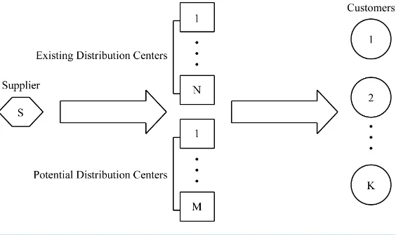
This paper investigates the competitive logistics distribution center location problem in uncertain environment. That is the problem in which a logistics company enters a market by locating a new distribution center where there are many existing distribution centers. The goal of the decision maker is to choose the location of the new distribution center so as to maximize its profit. The flow diagram of logistics distribution is shown in Figure 1. The potential distribution centers in Figure 1show that they can be selected to build a new distribution center. The setup costs of the potential distribution centers and the demands of customers are assumed to be uncertain variables with known uncertainty distributions. In addition, we assume that the customers patronize the nearest distribution center to meet their full demands.

3.2. Assumptions of Model

Before we begin to study competitive location problem with uncertain variables, we need to make some as-sumptions as follows (which are referred to Revelle [28] and Wu and Peng [27]):

1) There is one supplier and many existing distribution centers. 2) The supplier only supplies one kind of product.

3) There is no difference among the products provided by all distribution centers.

4) The location of the new distribution center can be selected from potential distribution centers.

5) The distances between the supplier and potential distribution centers, the distances between potential dis-tribution centers and customers and the distances between existing disdis-tribution centers and customers are known in advance.

6) The allocation of customers demands is related to the distance. The full demands of customers will be as-signed to the nearest distribution center.

In order to model the competitive location problem, we introduce the following indices and parameters: i: the index of existing distribution centers, i∈

{

1, 2,,N

}

;

j: the index of potential distribution centers, j∈

{

1, 2,,M

}

; k: the index of customers, k∈

{

1, 2,,K

}

;

c: the transportation cost of unit distance of the per product; w: the profit of the unit product;

j

d : the distance between the supplier and the j-th potential distribution center; jk

d : the distance between the j-th potential distribution center and the k-th customer; ik

D : the distance between the i-th existing distribution center and the k-th customer; j

h : the capacity of the j-th potential distribution center; k

ξ : the demand of the k-th customer, which is assumed to be an uncertain variable; k

Φ : the uncertainty distribution of ξ_k; j

η : the setup cost of the j-th potential distribution center, which is assumed to be an uncertain variable; j

[image:5.595.173.455.542.709.2]

Ψ : the uncertainty distribution of η_j;

(6)

j

x : the quantity supplied to the j-th potential distribution center from the supplier, which is a decision varia-ble;

jk

y : the quantity supplied to the k-th customer from the j-th potential distribution center, which is a decision variable;

j

ν : 0 - 1 variable implies whether the j-th potential distribution center is chosen to build the new distribution center or not.

Remark 1: The meaning of variable ν_j can be described as follows:

1, if the -th potential distribution center is chosen 0, otherwise.

j

j ν _{= }



In order to maximize the profit of the new distribution center, the decision maker must choose the appropriate site to build the new distribution center which attracts more customers. The majority of competitive location models assumed that customers will patronize the nearest distribution center. It is rationally for customers who want to sustain the less travel cost. In this paper, we consider that the customers choose the distribution center according to the distance between their sites and distribution centers rather than other conditions, such as price, service and attractiveness.

Thus we assume that the customers patronize the nearest distribution center, and this assumption which has been used by Revelle [28]. This patronizing behavior rule implies that the full demands of each customer are sa-tisfied by the nearest distribution center. The meaning of patronizing behavior which was proposed by Revelle [28] is listed in the following. If the new distribution center is nearer than all existing distribution centers, then the customers choose the new distribution center to satisfy their demands. If they have the same distance, then the half demands of customers are satisfied by the new distribution center. Otherwise, the customers choose the existing distribution center. In Revelle’s [28] model, the customers’ patronizing behavior is embodied in objec-tive function. It used two auxiliary variables to represent the facility which attracts full demands of customers and the facility which attracts half demands of customers, respectively. Our study is distinguished from the Re-velle’s [28] study by making the following important contribution: we use a function δ_jk to describe the cus-tomers’ patronizing behavior. Specifically, the expression of the function is listed in the following.

{ }

1

1, if min

1

, if min 2

0, otherwise.

jk ik i N jk jk ik

i N

d D

δ

≤ ≤

 <

 

=_ =

  

3.3. Expected Value Model

We note that the total profit of the new distribution center is made up of four parts. Thus the total profit is a function related to x, y and η, which can be written as

(

)

1 1 1 1 1 1

, ,

K M M K M M

j jk jk j j jk jk j j

k j j k j j

P x yη w ν δ y d x c d y c ν η

= = = = = =

=

∑∑

−

∑

−

∑∑

−

∑

where

(

1, , M

)

x= x  x

and

(

11, , 1K, , M1, , MK

)

y= y  y  y  y

are decision vectors, and

(

1, 2, , M

)

η

=

η η



η

(7)

Since we know the uncertain objective function P x y

(

, ,

η

)

cannot be directly maximized, we can maximize its expected value, i.e.,

(

)

,

max , , .

x y E P x y

η



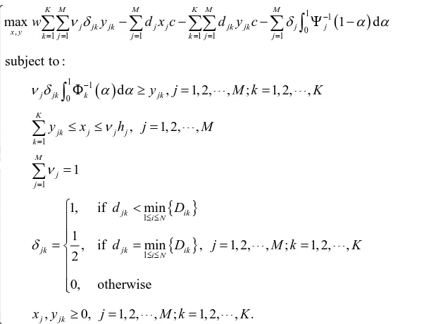
We employ the uncertain programming model to study the competitive logistics distribution center location problem. So we can build the expected value model as follow:

(

)

{ }

, 1 1 1 1

max , , .

subject to :

, 1, 2, , ; 1, 2, , , 1, 2, ,

1

1, if min

1

, if min , 1, 2, , ; 1, 2, , 2

0, otherwise , 0, 1, 2, ,

x y

j jk k jk K

jk j j j k M j j jk ik i N jk jk ik

i N

j jk

E P x y

E y j M k K

y x h j M

d D

d D j M k K

x y j M

η

ν δ ξ

ν ν δ = = ≤ ≤ ≤ ≤       ≥ = =   ≤ ≤ = =  <   = = = =    ≥ =

∑

    

 ;k 1, 2, ,K                       =   (1)

where δ ≠jk 0 and ν =j 1 show that xj >0 and yjk >0 for any j=1, 2,,M and k=1, 2,,K. Oth-erwise, xj =0 and yjk =0.

In this expected value model, the first constraint means that the quantity supply is not exceed the demand of customer. The second constraint implies the volume of transport is less than the capacity of the new distribution center. The third one shows that we select single site to build the new distribution center. And the last one en-sures the nonnegativity of decision variables x_j and y_jk.

4. The Crisp Equivalent Model

The key problem of the model is seeking for the optimal solution. Taking advantage of the operational law of uncertain variable, we can transform the expected value model (1) into its deterministic form. It is clearly that the total profit function is strictly decreasing with setup costs. According to Theorem 1 and Theorem 2, the ob-jective function

(

, ,

)

E P x y_ η _

can be converted into

(

)

1 ₁ 0

1 1 1 1 1 1

1 d .

K M M K M M

k j j k j j

w ν δ y d x c d y c δ − α α

= = = = = =

− − − Ψ −

∑∑

∑

∑∑

∑ ∫

(2)

Similarly, the first constraint

, 1, 2, , ; 1, 2, ,

j jk k jk

E_ν δ ξ  ≥_ y j=  M k=  K

can be turned into

( )

1 ₁

0 d , 1, 2, , ; 1, 2, , .

j jk k yjk j M k K

ν δ

_Φ−

α α

_≥ ₌ ₌

(8)

It follows from the formulas (2) and (3) that expected value model (1) can be switched to the following equivalent model:

(

)

( )

{ }

1 ₁ 0

, ₁ ₁ ₁ ₁ ₁ ₁

1 ₁ 0 1 1 1 1

max 1 d

subject to :

d , 1, 2, , ; 1, 2, ,

, 1, 2, ,

1

1, if min

1

, if min 2

K M M K M M

x y _k _j _j _k _j _j

j jk k jk

K

jk j j j

k M j j jk ik i N

jk jk i

i N

w y d x c d y c

y j M k K

y x h j M

d D

ν δ δ α α

ν δ α α

ν ν δ − = = = = = = − = = ≤ ≤ ≤ ≤

− − − Ψ −

Φ ≥ = =

≤ ≤ = = < = =

∑∑

∑

∑∑

∑ ∫

∫

∑

  

{ }

, 1, 2, , ; 1, 2, ,

0, otherwise

, 0, 1, 2, , ; 1, 2, , .

k

j jk

j M k K

x y j M k K

                   _ = =           ≥ = =      (4)

Clearly, we note that the equivalent model (4) is a deterministic programming model. As all know, the soft-ware Lingo cannot show the integral function. Therefore, we can find the optimal solution by using the mathe-matical software Matlab. In addition, in uncertainty theory, the inverse distribution function is easy to calculate for us. Thus we can calculate the inverse distribution function before we use the software Lingo to find the op-timal solution. We can choose one of them to solve this programming. For convenience, the following example is seeking for solution by Lingo.

5. Numerical Example

In order to illustrate the modeling idea and the effectiveness of this model, we give a numerical example in this section. Suppose that there is a supplier in a city. And there are 3 distribution centers to distribute the new model of the televisions to 7 customers. A logistics company want to select an optimal site from 4 potential distribution centers after survey. The distances dj, djk and Dik are listed in Table 1, Table 2 and Table 3, respectively. The unit transportation cost c = 0.01 and the unit product profit w = 5 are given via survey. ξ_k, η_j are assumed to be independent linear uncertain variables with known uncertainty distributions which are presented in Table 4

and Table 5, respectively. In addition, the capacities of potential distribution centers are listed in Table 4.

Table 1. The distance dj between supplier and potential distribution centers.

j 1 2 3 4

[image:8.595.173.474.114.344.2]

dj 150 200 210 170

Table 2. The distance Dik between existing distribution centers and customers.

i\k 1 2 3 4 5 6 7

1 10 20 30 28 15 15 25

2 14 25 25 32 30 12 20

[image:8.595.142.486.637.719.2]

(9)

[image:9.595.141.498.93.365.2]

Table 3. The distance djk between potential distribution centers and customers.

j\k 1 2 3 4 5 6 7

1 15 25 18 12 20 8 18

2 22 15 16 10 15 21 6

3 21 8 24 20 16 25 21

4 18 12 20 14 12 20 12

Table 4. The capacities hj and setup costs ηj of potential distribution centers.

j 1 2 3 4

j

h 200 240 180 210

j

[image:9.595.159.465.400.611.2]

η 

(

20, 24

)



(

24, 32

)



(

16, 20

)



(

22, 28

)

Table 5. The demands ξk of customers.

k 1 2 3 4 5 6 7

k

ξ (50, 56) (70, 76) (80, 90) (60, 76) (68, 72) (68, 72) (54, 60)

According to the model (4), the expected value model of this numerical example is listed in the following formula

(

)

( )

{ }

7 4 4 7 4 4 ₁ 1 0 ,

1 1 1 1 1 1

1 ₁ 0 7 1 4 1 1 3 1

max 5 0.01 0.01 1 d

subject to :

d , 1, 2, 3, 4; 1, 2, , 7 , 1, 2, 3, 4

1

1, if min

1

, if min 2

j jk jk j j jk jk j j x y

k j j k j j

j jk k jk jk j j j k j j jk ik i jk jk

y d x d y

y j k

y x h j

d D

d

ν δ δ α α

ν δ α α

ν δ δ − = = = = = = − = = ≤ ≤

− − − Ψ −

Φ ≥ = =

≤ ≤ = = < = =

∑∑

∑

∑∑

∑ ∫

∫

∑



{ }

3 , 1, 2, 3, 4; 1, 2, , 7 0, otherwise

, 0, 1, 2, 3, 4; 1, 2, , 7.

ik i

j jk

D j k

x y j k

≤ ≤                    ₌ ₌       _   ≥ = =    (5)

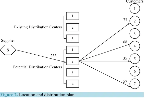
Then we use Lingo to get the optimal solution which is listed in the following.

22 32 42 14 24 25 16 17 27 47 1

1, 1, , 1, 1;

2

δ =δ =δ = δ =δ = δ = δ = δ =δ =δ =

1 3 4 0, 2 1;

ν =ν =ν = ν =

1 3 4 0, 2 233;

x =x =x = x =

22 73, 24 68, 25 35, 27 57.

(10)

[image:10.595.173.463.87.281.2]

Figure 2. Location and distribution plan.

The solution ν =₂ 1 shows that the second one is selected to build new distribution center, x2 = 233 means

that the supplier must supply 233 products to the new distribution center, and y22 = 73, y24 = 68, y25 = 35, y27 =

57, state that the quantity of product are supplied form new distribution center to customers. The above solutions show that we can choose the second potential distribution center to built the new distribution center and the total profit is 644.58. Meanwhile we can know how to distribute goods for customers according to the plan which is shown in Figure 2.

6. The Crisp Equivalent Model

In the process of practical logistics network optimization, uncertain factors often appear in competitive logistics distribution center location problem because of lacking of or even without historical data. This paper investi-gated a useful model to handle competitive logistics distribution center location problem with uncertain custom-ers demands and uncertain setup costs. The mathematical model of this problem was established by uncertain programming based on the expected value criterion. In order to solve this model, we took advantage of the properties of uncertain variable. Then the expected value model was transformed into its crisp equivalent model, and we used mathematical software Lingo to find its optimal solution. At last, a numerical example was pre-sented to illustrate the effectiveness of the proposed model.

This paper only considers the demands of customers and setup costs of new distribution center are uncertain variables. Indeed, other uncertain factors in competitive logistics distribution center location problem are worthy of studying. We can further focus on the uncertain utility which can be used to describe the uncertainty of cus-tomers’ patronizing behavior. Furthermore, we can seek for the expression of uncertain utility. In this paper, we only center on the static competition. It is necessary for further research to consider dynamic competition prob-lem. Thus we can establish dynamic uncertain programming model for uncertain dynamic competitive facility location problem.

Acknowledgements

This work was supported by the Projects of the Humanity and Social Science Foundation of Ministry of Educa-tion of China (No. 13YJA630065), and the Key Project of Hubei Provincial Natural Science FoundaEduca-tion (No. 2012FFA065).

References

[1] Lu, A. and Bostel, N. (2007) A Facility Location Model for Logistics Systems including Reverse Flows: The Case of Remanufacturing Activities. Computers & Operations Research, 34, 299-323.

http://dx.doi.org/10.1016/j.cor.2005.03.002

(11)

[3] Hotelling, H. (1929) Stability in Competition. Economic Journal, 39, 41-57. http://dx.doi.org/10.2307/2224214

[4] Drezner, Z. (1982) Competitive Location Strategies for Two Facilities. Regional Science and Urban Economics, 12, 485-493. http://dx.doi.org/10.1016/0166-0462(82)90003-5

[5] Hakimi, S. (1983) On Locating New Facilities in a Competitive Environment. European Journal of Operational Re-search, 12, 29-35. http://dx.doi.org/10.1016/0377-2217(83)90180-7

[6] Plastria, F. (2001) Static Competitive Facility Location: An Overview of Optimisation Approaches. European Journal of Operational Research, 129, 461-470. http://dx.doi.org/10.1016/S0377-2217(00)00169-7

[7] Wong, S. and Yang, H. (1999) Determining Market Areas Captured by Competitive Facilities: A Continuous Equili-brium Modeling Approach. Journal of Regional Science, 39, 51-72. http://dx.doi.org/10.1111/1467-9787.00123

[8] Yang, H. and Wong, S. (2000) A Continuous Equilibrium Model for Estimating Market Areas of Competitive Facili-ties with Elastic Demand and Market Externality. Transportation Science, 34, 216-227.

http://dx.doi.org/10.1287/trsc.34.2.216.12307

[9] Plastria, F. and Vanhaverbeke, L. (2008) Discrete Models for Competitive Location with Foresight. Computers & Op-erations Research, 35, 683-700. http://dx.doi.org/10.1016/j.cor.2006.05.006

[10] Küçükaydin, H., Aras, N. and Altnel, I. (2012) A Leader-Follower Game in Competitive Facility Location. Computers & Operations Research, 39, 437-448. http://dx.doi.org/10.1016/j.cor.2011.05.007

[11] Sasaki, M., Campbell, J., Krishnamoorthy, M. and Ernst, A. (2015) A Stackelberg Hub Arc Location Model for a Competitive Environment. Computers & Operations Research, 47, 27-41.

http://dx.doi.org/10.1016/j.cor.2014.01.009

[12] Drezner, T. (1994) Locating a Single New Facility among Existing Unequally Attractive Facilities. Journal of Regional Science, 34, 237-252. http://dx.doi.org/10.1111/j.1467-9787.1994.tb00865.x

[13] Drezner, T., Drezner, Z. and Kalczynski, P. (2011) A Cover-Based Competitive Location Model. Journal of the Oper-ational Research Society, 62, 100-113. http://dx.doi.org/10.1057/jors.2009.153

[14] Huff, D. (1966) A Programmed Solution for Approximating an Optimum Retail Location. Land Economics, 42, 293- 303. http://dx.doi.org/10.2307/3145346

[15] Drezner, T. (2014) A Review of Competitive Facility Location in the Plane. Logistics Research, 7, 114-126.

http://dx.doi.org/10.1007/s12159-014-0114-z

[16] Leonardi, G. and Tadei, R. (1984) Random Utility Demand Models and Service Location. Regional Science and Urban Economics, 14, 399-431. http://dx.doi.org/10.1016/0166-0462(84)90009-7

[17] Drezner, T. and Drezner, Z. (1996) Competitive Facilities: Market Share and Location with Random Utility. Journal of Regional Science, 36, 1-15. http://dx.doi.org/10.1111/j.1467-9787.1996.tb01098.x

[18] Drezner, T., Drezner, Z. and Wesolowsky, G. (1998) On the Logit Approach to Competitive Facility Location. Journal of Regional Science, 38, 313-327. http://dx.doi.org/10.1111/1467-9787.00094

[19] Shiode, S. and Drezner, Z. (2003) A Competitive Facility Location Problem on a Tree Network with Stochastic Weights. European Journal of Operational Research, 149, 47-52. http://dx.doi.org/10.1016/S0377-2217(02)00459-9

[20] Drezner, Z. and Wesolowsky, G. (1981) Optimal Location Probabilities in the p Distance Weber Problem.

Trans-portation Science, 15, 85-97. http://dx.doi.org/10.1287/trsc.15.2.85

[21] Shiode, S. and Ishii, H. (1991) A Single Facility Stochastic Location Problem under a Distance. Annals of Operations Research, 31, 469-478. http://dx.doi.org/10.1007/BF02204864

[22] Wesolowsky, G. (1977) Probabilistic Weights in the One Dimensional Facility Location Problem. Management Science, 24, 224-229. http://dx.doi.org/10.1287/mnsc.24.2.224

[23] Liu, B. (2007) Uncertainty Theory. Spinger-Verlag, Berlin. http://dx.doi.org/10.1007/978-3-540-73165-8_5

[24] Gao, Y. (2012) Uncertain Models for Single Facility Location Problems on Networks. Applied Mathematical Model-ling, 36, 2592-2599. http://dx.doi.org/10.1016/j.apm.2011.09.042

[25] Wen, M., Qin, Z. and Kang, R. (2014) The α-Cost Minimization Model for Capacitated Facility Location-Allocation Problem with Uncertain Demands. Fuzzy Optimization and Decision Making, 13, 345-356.

http://dx.doi.org/10.1007/s10700-014-9179-z

[26] Wang, K. and Yang, Q. (2014) Hierarchical Facility Location for the Reverse Logistics Network Design under Uncer-tainty. Journal of Uncertain Systems, 8, 255-270.

[27] Wu, Z. and Peng, J. (2014) A Chance-Constrained Model of Logistics Distribution Center Location under Uncertain Environment. Advances in Information Sciences and Service Sciences, 6, 33-42.

(12)

Journal of Regional Science, 26, 343-358. http://dx.doi.org/10.1111/j.1467-9787.1986.tb00824.x

[29] Liu, B. (2010) Uncertainty Theory: A Branch of Mathematics for Modeling Human Uncertainty. Spinger-Verlag, Ber-lin. http://dx.doi.org/10.1007/978-3-642-13959-8

[30] Liu, B. (2009) Some Research Problems in Uncertainty Theory. Journal of Uncertain Systems, 3, 3-10.