Heterogeneous Convergence

Munich Personal RePEc Archive

Heterogeneous Convergence

Young, Andrew and Higgins, Matthew and Levy, Daniel

West Virginia University, Georgia Institute of Technology, and

Bar-Ilan University and Emory University

25 October 2006

Online at

https://mpra.ub.uni-muenchen.de/46038/

Heterogeneous Convergence

Andrew T. Young a,, Matthew J. Higgins b,c, Daniel Levy d, e, f

a

College of Business and Economics, West Virginia University, Morgantown WV 26506, USA

b

Scheller College of Business, Georgia Institute of Technology, Atlanta, GA 30308, USA

c _{National Bureau of Economic Research, Cambridge, MA 02138 USA}

d

Department of Economics, Bar-Ilan University, Ramat-Gan 52900, ISRAEL

e

Department of Economics, Emory University, Atlanta, GA 30322, USA

f

Rimini Center for Economic Analysis, Rimini, ITALY

Last Revision: April 2013

______________________________________________________________________________________

Abstract_{: We use U.S. county-level data to estimate convergence rates for 22 individual}

states. We find significant heterogeneity. E.g., the California estimate is 19.9 percent and the New York estimate is 3.3 percent. Convergence rates are essentially uncorrelated with income levels.

______________________________________________________________________________________

JEL Codes: O40, O11, O18, O51, R11, H50, H70

Key Words: Economic Growth, Conditional Convergence, Heterogeneity, U.S. County Level Data

 _{We are grateful to the referee for constructive comments that helped us improve the manuscript. We thank Steven}

Durlauf, Jordan Rappaport and Jerry Thursby for helpful comments and suggestions and Paul Evans for answering our questions. We are grateful to Jordan Rappaport for kindly sharing with us data and computer codes. Matthew Higgins acknowledges financial assistance from a National Science Foundation IGERT Fellowship and The Imlay Professorship. Daniel Levy gratefully acknowledges financial support from Adar Foundation of the Economics Department at Bar-Ilan University. All errors are our own.



Corresponding author: [email protected], Tel: 304-2934526

1

1. Introduction

Empirical conditional convergence studies implicitly assume that all economies follow

identical growth processes and that, therefore, it is meaningful to estimate a single rate of convergence. However, Evans (1998) argues that this is implausible for most data sets because countries (p. 296) "… have different technologies, preferences, institutions, market structures, etc."1

We use county-level data from 22 individual states, comprising a total of 1,921 U.S. counties to study heterogeneity in convergence rates. The data include per capita income

growth and 29 other conditioning variables. Conditional on the latter, we report separate convergence rate estimates for each of these 22 states.

Existing studies of heterogeneity in growth represent a range of ingenious econometric techniques designed to cope with a limited number of observations typically available for growth studies.2 Given the richness of our data, we are able to explore heterogeneity in

convergence rates amongst the U.S. states by incorporating a large number of demographic and socio-economic variables as controls.

Our data offer several other advantages. A single institution collects it, ensuring uniform variable definitions. There is no exchange rate variation between the counties and the price variation across counties is smaller than across countries, reducing the

potential errors-in-variables bias (Bliss, 1999).3 Counties within a state form a sample with geographical homogeneity and a shared state government. To a great extent the states are ready-made “clubs” within which we would expect convergence. The large data set allows us to study inter-state heterogeneity, while the intra-state homogeneity

increases the accuracy likelihood of the specification we employ.

There are considerable per capita income differences across U.S. states. While Higgins

et al. (2006) find that U.S. county-level data is well-described by conditional

convergence, Young et al. (2008), using the same data, find that the actual dispersion of income levels is not decreasing. One possible explanation for this is that many individual states are not well-described by conditional convergence. Another possibility is that

poorer economies have relatively low convergence rates. State-specific convergence rate

1

Levy and Dezhbakhsh (2003) provide international evidence on output fluctuation and shock persistence that may be considered an indirect evidence of such heterogeneity.

2

See, e.g., Durlauf and Johnson (1995), Lee et al. (1997), Rappaport (2000), Brock and Durlauf (2001), Durlauf et al. (2001), and Rodrik (2013). See also the “club convergence” literature. For example, Quah (1996, 1997), Desdoigts (1999), and Canova (2004).

3

estimates can help in assessing the plausibility of this explanation.

We find significant heterogeneity in the state-level convergence rates. Across the 22

states, we obtain a range of point estimates including 2.7 percent (Georgia) and 19.9 percent (California). The average convergence rate across these states is 9.2 percent. We also find that convergence rates and income levels are essentially uncorrelated,

suggesting that poorer states are not at an inherent disadvantage in catching up to their richer counterparts.

The paper is organized as follows. Section 2 discusses the model and our estimation

strategy. Section 3 describes the data. Section 4 reports the findings. Section 5 concludes.

2. Econometric model

As Barro and Sala-i-Martin (1992) show, the neoclassical growth model implies that

n n n

n y x

g 









economy n between years 0 and T,  is a function of the exogenous rate of technical

progress, and





e T

 _{ } 

with B representing the responsiveness of the average

growth rate to the gap between the steady state income and the initial value, y_n0; x_n0 is a

vector of control variables,  is a coefficients' vector, and



variance error term.

We adapt the basic growth model to panel data:

nt t nt nt

nt y x

g  ,0   , (1)

where t indexes T = 5 year intervals that will begin, in our data, at 1970, 1975, 1980, 1985, 1990, 1995, 2000, and 2005, and φt is a period fixed effect. For example, the first

observation for a county n, will consist of gn,1970 (yn,1975 yn,1970)/5, yn,1970, and xn,1970.

We estimate (1) using generalized method of moments (GMM) including period fixed

effects. Based on the estimate, ˆ , we calculate the convergence rate point estimate as





T

c11 ˆ1 . To calculate a 95 percent confidence interval we compute





ˆ_{ se}

 , where s.e. is the standard error of ˆ . If the low value of the confidence

3

3. U.S. county-level data

We begin with U.S. county level data that include 3,057 county-level observations

covering all 50 states from 1970 to 2010. However, statistically significant convergence rates estimates can only be computed for 22 states (constituted by 1,921 counties). We use the log of real per capita personal income net of transfers. We also start with 29 conditioning variables that correspond approximately to the set used by Higgins, et al. (2006, 2009, 2010) and Young, et al. (2008).4 The panel has a time dimension of 8.

Our identification strategy is to use lagged control variables as instruments. We

initially run an OLS, period fixed effects regression of growth on initial income and all of the other controls. From that regression we identify 7 controls that are statistically

insignificant. Of those we choose 4 to use as excluded instruments that create over-identification in our GMM estimations.5 This decreases our time dimension to 7.

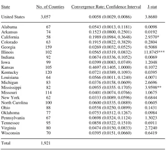
4. Convergence rate estimates

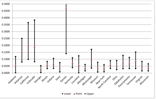
Table 1 reports the asymptotic conditional convergence rate estimates with 95 percent confidence intervals for 22 individual U.S. states. Figure 1 presents confidence intervals as vertical bars around the point estimates. The individual state estimates vary

significantly, indicating cross-state heterogeneity. The average estimate for the 22-state

sample is 9.2 percent and for 4 states the point estimate exceeds 10 percent.6 Table 1 also reports J-statistics. At better than the 10 percent level the over-identifying restrictions are rejected only 3 times; only 2 times at better than the 5 percent level.

Thus, there is considerable heterogeneity in the estimated convergence rates. The full picture that one gets from Table 1and Figure 1is of a group of economies with high

4

The conditioning variables are collected at the county level and include: land and water area per capita; percentage of 5–13, 14–17, 18–64, and 65+ year olds; percentage of blacks and Hispanics; percentage of population with education of 9–11 years, high school diploma, some college, and bachelor degree or more; percentage of population below the poverty line; percentage of the population employed by federal, state, and local governments; percentage of self-employed; percentage of population employed in agriculture-fishing-and-forestry, construction, services, finance-insurance-and-real-estate, manufacturing, mining, retail, transportation and public utilities, wholesale trade, college town and metro area indicators. The few differences in the control variable set used here versus Higgins et al. (2006) are the result of moving from a cross section of growth from 1970 to 1998 to the updated panel used here, from 1970 to 2005. This required using BEA rather than Census data. The BEA, for example, collapses some industry categories into a single category and redefines others.

5

Caselli, et al. (1996) suggest GMM estimation based on first differencing the growth equation. Bond, et al. (2001) suggest estimating a system including the first-differenced equation. We focus on the un-differenced growth equation because our controls represent evolving characteristics of economies; most of the information is in the levels. The excluded instruments are the college town indicator, the land area per capita, and the population percentages employed in transportation and public utilities and in wholesale trade. Of the other three not-significant controls from the OLS regression, two were educational attainment variables. The other was federal government employment that Higgins et al. (2010) find to be a robust correlate of growth.

6

(typically above 5 percent) but often quite different rates of convergence. This

heterogeneity should not be surprising. The convergence rate in the neoclassical growth

model is a function of the technology and population growth rates, the depreciation rate, and the technology and preference parameters. Therefore, differences in the particular industries that predominate in an economy, cultural characteristics, and institutions may translate into different convergence rates.

A simple OLS regression of the state convergence rate point estimates on average per capita income levels yields a partial correlation of 0.1677 and it not statistically

significant. This suggests that poorer economies are not in general facing relatively poor convergence potentials.

5. Conclusions

We use 1,921 U.S. county-level observations to explore the variation in income

convergence across the U.S. states. Across 22 individual states, the estimated

convergence rates average 9.2 percent. For 15 states the point estimate convergence rate is above 5 percent. We find substantial heterogeneity in individual state convergence rates.

The high convergence rates are encouraging in the sense that, given proper policies to

induce and support balanced growth paths, laggard economies can close the gap relatively quickly. Convergence rates are, in principle, functions of deep technology and preference parameters. If these deep parameters differ enough across U.S. states to create

5

References

Barro, R.J., Sala-I-Martin, X., 1991. Convergence across states and regions. Brookings Papers on Economic Activity 1, 107–158.

Barro, R.J., Sala-i-Martin, X., 1992. Convergence. Journal of Political Economy 100, 223–251.

Bliss, C., 1999. Galton’s fallacy and economic convergence. Oxford Economic Papers 51, 4–14.

Bond. S., Hoeffler, A., Temple, J., 2001. GMM estimation of empirical growth models. CEPR Discussion Paper 3048.

Brock, W.A., Durlauf, S.N., 2001. Growth empirics and reality. World Bank Economic Review 15, 229–272.

Canova, F., 2004. Testing for convergence clubs in income per capita: a predictive density approach. International Economic Review 45, 49–77.

Casseli, F., Esquivel, G., Lefort, F., 1996. Reopening the convergence debate: a new look at cross-country growth regressions. Journal of Economic Growth 1, 363–389.

Desdoigts, A., 1999. Patterns of economic development and the formation of clubs. Journal of Economic Growth 4, 305–330.

Durlauf, S.N., Johnson, P.A., 1995. Multiple regimes and cross-country growth behavior. Journal of Applied Econometrics 10, 365–384.

Durlauf, S.N., Kourtellos, A., Minkin, A., 2001. The local Solow growth model. European Economic Review 45, 928–940.

Evans, P., 1997a. How fast do economies converge? Review of Economics and Statistics 36, 219–225.

Evans, P., 1997b. Consistent estimation of growth regressions. Unpublished manuscript, available at http://economics.sbs.ohiostate.edu/pevans/pevans.html.

Evans, P., 1998. Using panel data to evaluate growth theories. International Economics Review 39, 295–306.

Higgins, M., Levy, D., Young, A.T., 2006. Growth and convergence across the U.S: evidence from county-level data. Review of Economics and Statistics88(4), 671–681. Higgins, M., Young, A.T., Levy, D., 2009. Federal, state and local governments:

evaluating their separate roles in the US growth. Public Choice139, 493–507. Higgins, M., Young, A.T., Levy, D., 2010. Robust correlates of county-level growth in

the United States. Applied Economics Letters 17(3), 293–296.

Lee, K., Pesaran, M.H., Smith, R., 1997. Growth and convergence in a multi-country empirical stochastic growth model. Journal of Applied Econometrics 12, 357–384. Levy, D., Dezhbakhsh, H., 2003. International evidence on output fluctuation and shock

persistence. Journal of Monetary Economics 50, 1499–1530.

Quah, D.T., 1996. Twin peaks: growth and convergence in models of distributional dynamics. Economic Journal 106, 1045–1055.

Quah, D.T., 1997. Empirics for growth and distribution: stratification, polarization, and convergence clubs. Journal of Economic Growth 2, 27–59.

Rappaport, J., 2000. Is the speed of convergence constant? Working Paper No. 00-10, Federal Reserve Bank of Kansas City.

Rodrik, D., 2013. Unconditional convergence in manufacturing. Quarterly Journal of Economics 128, 165–204.

Fig. 1. Point estimates of the within-state asymptotic convergence rates with 95% confidence intervals

0.0000 0.0500 0.1000 0.1500 0.2000 0.2500 0.3000 0.3500 0.4000 0.4500 0.5000

7

Table 1

Asymptotic conditional convergence rates for 22 U.S. States using GMM: Point estimates with 95% confidence intervals

State No. of Counties Convergence Rate; Confidence Interval J-stat United States 3,057 0.0058 (0.0029, 0.0086) 3.8680 Alabama 67 0.0543 (0.0013, 0.1181) 0.0098 Arkansas 74 0.1523 (0.0800, 0.2501) 0.0192 California 58 0.1989 (0.0984, 0.3648) 2.9370* Colorado 63 0.1915 (0.0822, 0.3829) 0.2804 Georgia 159 0.0269 (0.0032, 0.0525) 0.5088 Illinois 102 0.0565 (0.0319, 0.0832) 11.8745*** Indiana 92 0.0674 (0.0336, 0.1052) 0.0069 Iowa 99 0.0399 (0.0083, 0.0749) 1.2048 Kansas 105 0.4697 (0.1405, 1.0000) 0.1072 Kentucky 120 0.0721 (0.0389, 0.1093) 0.0395 Louisiana 64 0.0566 (0.0011, 0.1240) 4.0071 Michigan 83 0.0376 (0.0158, 0.0609) 2.6696 Mississippi 82 0.0955 (0.0355. 0.1705) 3.9598** Missouri 114 0.0401 (0.0074, 0.0766) 1.0675 New York 62 0.0333 (0.0089, 0.0596) 0.6844 North Carolina 100 0.0600 (0.0335, 0.0889) 0.0605 Ohio 88 0.0558 (0.0250, 0.0899) 0.1431 Oklahoma 77 0.0753 (0.0312, 0.1267) 0.0984 Pennsylvania 67 0.0698 (0.0324, 0.1124) 1.3023 Tennessee 95 0.0858 (0.0322, 0.1510) 0.6911 Virginia 80 0.0474 (0.0150, 0.0833) 2.7240 Wisconsin 70 0.0395 (0.0151, 0.0660) 0.6419 Total 1,921