An aggregate import demand function for Turkey: a cointegration analysis

Munich Personal RePEc Archive

An aggregate import demand function

for Turkey: a cointegration analysis

Kalyoncu, Huseyin

April 2006

Online at

https://mpra.ub.uni-muenchen.de/4260/

An Aggregate Import Demand Function for Turkey: A Cointegration Analysis

Huseyin KALYONCU*

Department of Economics, University of Cukurova TURKEY

ABSTRACT

This paper estimates an aggregate import demand function for Turkey during the period 1994:1-2003:12. In our empirical analysis of the aggregate import demand function for Turkey, cointegration and error correction modelling approaches have been used. Empirical results suggest that there exists a unique long-run or equilibrium relationship among real quantities of imports, relative import price and real GNP.

I. INTRODUCTION

The demand for imports in an economy is a crucial macroeconomic relationship with significant implications for the design and conduct of economic policy. In this paper, we

intend to determine whether there exist a long-run relationship between Turkey’s aggregate import volume and its major determinants, on the basis of monthly data for the period

1994-2001. First, the hypothesis of the existence of a cointegrated relationship between aggregate import volume and its major determinants is tested using cointegration technique developed by Engle- Granger (1987), Johansen (1988,1991) and Johansen-Juselius (1990, 1992 and 1994). If the hypothesis of no cointegration is rejected, a stable long-run relationship between the aggrageta import demand function and its major determinants exist. Secondly, we attempt to estimate an error-correction model (ECM) to integrate the dynamics of short-run (changes) with long run (levels) adjustment processes.

The remainder of this paper is organized as follows. In the second part, some empirical studies on the estimation of the import demand function are discussed. The import demand function for Turkey is modeled in the third part. After that the empirical results are reported and discussed. The last part concludes the paper.

* _{Faculty of Economics and Administrative Sciences, Depatrment of Economics, Cukurova University, P.O.}

II. LITERATURE

In the study by Deyak, et al. (1989), the stability of the U.S. aggregate and disaggregated

import demand functions were considered. These functions are estimated by OLS from 1958:Q4 to 1983:Q4. Import demand is disaggregated by economic class: crude foods, crude materials, manufactured foods, semi-manufactured foods, and finished manufactures. Except for the crude materials, estimated price elasticities have the correct negative sign and they are statistically significant. For the income elasticities, the significant positive sign is estimated again except for the crude materials. The coefficient of the lagged dependent variable is also significantly positive.

Dutta and Ahmed (1997) study Bangladesh import performance and use quarterly data for the period 1974-1994. They applied cointegration and error correcting modeling approaches and find unique equilibrium relationship exists among the real quantity of imports, real import prices, real GDP and real foreign exchange reserves. They applied two types of error correction models (ECMs): one based on lagged residuals from a static cointegrating

regression equation and the other through a vector autoregression method The error correction term in both the models has been found to be statistically significant, suggesting the validity

of the long-run equilibrium relationship. Estimated price elasticities have the correct negative sign and they are statistically significant. For the income elasticities, the significant positive sign is estimated and they are also significant.

Sinha (1997) estimates an aggregate import demand function for Thailand using annual data for the period, 1953-90. Using the cointegration approach, he find aggregate import demand for Thailand to be price inelastic, cross price inelastic (with respect to domestic price) and income inelastic in the short run. In the long run, aggregate import demand is still price inelastic and cross price inelastic. However, aggregate import demand is highly income elastic in the long run.

individually and jointly tested. Also, the short run elasticities of the two models are compared. The first model estimates imports using the Engle-Granger approach. It is found that in the long run, income level, nominal depreciation rate, inflation rate and international reserves significantly affect imports. The second approach models import demand using the Bernanke-Sims structural VAR method. The findings indicate that anticipated changes in the real depreciation rate and unanticipated changes in the income growth and real depreciation rate have significant effects on import demand growth.

A disequilibrium monetary model is constructed as a quarterly macroeconometric model for Turkey by Özatay(1997). The 1977:Q1-1996:Q4 period is covered in the estimation. The model is estimated by two-step procedure of Engle-Granger methodology. Total imports of goods in US dollars are explained as a function of real income and real exchange rate. The hypothesis is the existence of long run relationships between the level of real imports and real manufacturing output, real total investments and real exchange rate. The short run dynamics is modeled as an adjustment to this long run relationship. In the long run, income is found to be significant but it loses its significance in the short run. There is a correction to the long run equilibrium every period in the short run. Real exchange rate is negatively influencing total

imports of goods, both in the long and short run.

Erlat and Erlat (1991) study Turkish export and import performance and use annual data for the period 1967-87. Export supply, export demand and import demand functions are estimated by OLS first, then three equations are estimated as a set of seemingly unrelated regressions. Total volume of imports is regressed on domestic real income, price of imports (including tariffs) divided by domestic prices, real international reserves and one period lagged value of the dependent variable. Two dummies are introduced for the years 1978 and 1979 to explain the structural shift. International reserves are found to be the most important variable in explaining import demand. Relative prices, however, have no significant explanatory power on import demand.

In the study by Saygılı, et al. (1998), long run and short run export and import functions are

the most significant variable in the explanation of imports. Results show that short run income elasticity of imports is significant and 0.85. In the short run, real effective exchange has a significant coefficient with the expected sign but in the long run, it loses its significance on imports.

III. THEORY

Mayes (1981) give a simple import demand function. The volume of imports, M, is thought to depend upon the level of real economic activity in the importing country, Y, and the relative price of imports to domestic products, PM/PD, in the form

c b

PD PM Y a

M= ( / ) 1

This can be estimated readily by logarithmic transformation

u PD PM c

Y b a

M= + log + log( / ) +

log ₀ 2

where ao =log a and u is the error term. The coefficients b and c represent the income and

price elasticities of import demand respectively. It is expected that b>0 and c<0.

Econometric investigations of import demand also postulate that the demand for imports is a function of relative prices and real income (Houthakker and Magee, 1969; Le amer and Stern, 1970; Murray and Ginman, 1976; Goldstein and Khan, 1985; and Carone, 1996). Studies by Khan and Ross (1977) and Salas (1982) suggest that in modeling an aggregate import demand function, the log-linear specification is preferable to the linear formulation. Thus we use the log-linear specification to estimate import demand function for Turkey.

IV. EMPIRICAL RESULTS

4.1. Data

Let M be real imports (first monthly import estimates, converted to their TL by using the average USD exchange rate over the month second imports in millions of TL divided by the

4.2.Unit-Root Tests

In this section we analyze the time-series properties of the data during the period 1994 –2001. We have conducted the Augmented Dickey-Fuller (ADF) and Phillips-Perron (PP) unit root tests. These unit-root tests are performed on both levels and first differences of all the three variables.

The ADF tests (Table 1) and the PP test (Table 2) confirm stationary for all the three variables (LNM, LNY, LN(PM/PD)). However, first differencing of all the variables shows stationary under the tests.

Table 1 : ADF unit root test for stationary

I0

Variables With trend Without trend No trend no constant Critical Value

LNM -1.48599 (4) -1.45217 (4)

LNY -2.19353 (12) -2.46532 (12) -0.05014 (12) LN(PM/PD) -0.91293 (4) -0.39079 (4)

-3.41 -2.86 -1.95

I1

Variables With trend Without trend No trend no constant Critical Value

LNM -6.75191 (4)

LNY -2.71467 (12) -2.15987 (12) -2.24880 (12) LN(PM/PD) -3.76025 (4)

-3.41 -2.86 -1.95

Notes : (i) Unit root tests were performed using Winrats.

(ii) figures in bracket indicate lag order and the lag order was determined using the Schwarz criterion (BIC). (iii) 95% critical values for ADF statistics in order with trend, without trend, no trend no constant.

Table 2 : Phillips-Perron (PP) unit root test for stationary

I0

Variables With trend Without trend No trend no constant Critical Value

LNM -3.018785 -1.526820 5.030468 LNY -4.957140 -4.844017 0.006606

LN(PM/PD) -1.130994 -1.221189 5.252092

-3.45 -2.89 -1.94

I1

Variables With trend Without trend No trend no constant Critical Value

LNM -14.95065 -14.68881 -11.41769

LNY -11.58391 -11.58858 -11.65106

LN(PM/PD) -10.10056 -10.10056 -4.787341 -1.94

Notes : (i) Unit root tests were performed using Eviews 3.0. (ii) Newey-West suggest 3 lag order.

(iii) 95% critical values for ADF statistics in order with trend, without trend, no trend no constant.

4.3.Cointegration Tests

In this section we have conducted the Engle-Granger’s (EG) Residual-based ADF test and

Johansen-Juselius (JJ) method.

As the first step of the EG cointegration test, we estimated Equation (2) using the OLS method. Second step of the EG procedure and check the stationarity of residuals by using the ADF test. The result are presented in Table 3 below.

Table 3. Engle-Granger Cointegration Tests

ADF(13) -2.75 (-1.94)

Notes: (i) Figures in bracket indicate 95 percent critical values. (ii) Lag order was determined using the Schwarz criterion (BIC).

At the 5 per cent level of significance, the ADF(13) statistic suggests rejecting the hypothesis of no-cointegration. There is one cointegrating relationship involving three variables.

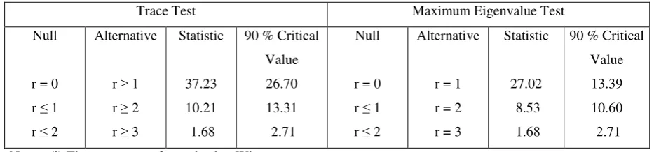
When there are more than two variables the JJ procedure provides more robust results. Before undertaking cointegration tests, let us first specify the relevant order of lags(p) of the Vector Autoregression (VAR) model. Lag order was determined using the Schwarz criterion. Lag in VAR model is 9. The results obtained from the JJ method are presented in Table 4 below.

Table 4. Johansen-Juselius Maximum Likelihood Cointegration Tests

Trace Test Maximum Eigenvalue Test

Null

r = 0 r 1 r 2

Alternative

r 1 r 2 r 3

Statistic

37.23 10.21 1.68

90 % Critical Value 26.70 13.31 2.71

Null

r = 0 r 1 r 2

Alternative

r = 1 r = 2 r = 3

Statistic

27.02 8.53 1.68

90 % Critical Value 13.39 10.60 2.71

Starting with the null hypothesis of no cointegration (r=0) among the variables, the trace statistic is 37.23, which is well above the 90 per cent critical value of 26.70. Hence it rejects the null hypothesis r =0, in favour of the general alternative r 1. As is evident in Table 4, the null hypothesis of r 1, r 2 can not be rejected at a 10 percent level of significance. Consequently, we can conclude that there is only one cointegrating relationship involving three variables of LNM, LNY and LN(PM/PD).

Turning to the maximum eigenvalue test, the null hypothesis of no cointegration (r=0) is rejected at a 10 percent level of significance in favour of the specific alternative, that there is one cointegrating vector, r=1. However, the test fails to reject the null hypothesis of r 1, r 2. This confirms the conclusion that there is only one cointegrating relationship amongst the three variables.

Thus, both the trace and the maximum eigenvalue test statistics reject the null hypothesis of r=0 at the 10 percent level of significance, and suggest that there is unique cointegrating vector. Therefore, our monthly data from 1994 to 2001 appear to support the proposition that in Turkey there exist a stable long-run relationship of aggregate import demand with its major determinants.

Estimates of long-run cointegrating vectors are given in Table 5.

Table 5. Estimates Of Long-Run Cointegrating Vectors

LNM 1.00

LNY -2.281

LN(PM/PD) 1.145 Notes: (i) The test was performed using Winrats.

(ii) The long-run equilibrium relation is: LNM = 2.281 LNY – 1.145 LN(PM/PD)

4.4.Estimation of Error-Correction Model

Following Hendry’s (1995) general-to-specific modelling approach, we first include 12 lags of the explanatory variables and 1 lag of the error correction (EC) term, and then gradually

T T N

N

T LNY LN PM PD EC

LNM =β + β ∆ + β ∆ +β +ε

∆ ₋

= =

1 3 0

2 0

1

0 ( / )

3

After experimenting with the general form of the ECM, the following model is found to fit the data best (Table 6):

Table 6: Estimated Error-Correction Model

Dependent Variable: ∆LNM

Regressors Parameter Estimates T-Ratio

∆LNY(-6)

∆LN(PM/PD) EC(-1)

-0.88 -1.07 -0.28

-6.66 -2.86 -3.39

Adj R2 _{= 0.47}

D.W. = 2.38 LM = 7.6 RESET= 0.25 NORMAL TY= 2.57 HET = 24.8

V. CONCLUSION

In our empirical analysis of the aggregate merchandise import demand function for Turkey, cointegration and error correction modeling approaches have been used. We find a unique equilibrium relationship exist among the real quantity of imports, relative prices and real GNP. In the estimated ECM, relative prices and real GNP (lagged six month) have all

emerged as important determinants of the import demand function for Turkey. The estimated coefficient of the error correction term (-0.28) indicates speed of adjustment to equilibrium.

Our econometric estimates of the aggregate merchandise import demand function for Turkey suggest that imports are sensitive to relative import prices changes (-1.07). the value of income elasticity of demand for imports lagged six month is –0.88. Thus, price elasticities of demand for imports is greater than income elasticities.

REFERENCES

Carone, G. (1996), “Modeling the U. S. Demand for Imports Through Cointegration and Error Correction,” Journal of Policy Modeling, 18(1):1-48.

Deyak, T.A., Sawyer, W.C. and Sprinkle, R.L., 1989, “An Empirical Examination of the Structural Stability of Disaggregated U.S. Import Demand,” The Review of Economics and Statistics, 71, pp. 337-341.

Dutta, D. and N. Ahmed (1997), “An Aggregate Import Demand Function for Bangladesh: A Cointegration Approach,” Applied Economics, 31(1999):465-472.

Engle, R.F. and Granger, C.W.J., 1987, “Cointegration and Error Correction: Representation, Estimation and Testing,” Econometrica, 55, pp. 251-76.

Erlat, G. and Erlat, H., 1991, “An Empirical Study of Turkish Export and Import Function,” CBRT and METU.

Goldstein, M. and M. S. Khan (1985), “Income and Price Effects in Foreign Trade,” in R. W. Jones and P. B. Kenen (eds.) Handbook of International Economics (Vol. II), New York:

Elsevier Science Publications, 1041-1105.

Hendry, D. F. (1995), Dynamic Econometrics, Oxford: Oxford University Press. International

Monetary Fund, International Financial Statistics (various issues).

Houthakker, H. S. and S. P. Magee (1969), “Income and Price Elasticities in World Trade,”

Review of Economics and Statistics, 41:111-25.

Johansen, S. (1988), “Statistical Analysis of Cointegrating Vectors,” Journal of Economic Dynamics and Control, 12: 231-54.

–––––––––– (1991), “Estimation and Hypothesis Testing of Cointegration Vectors in Gaussian Vector Autoregressive Models,” Econometrica , 59: 1551-80.

–––––––––– and K. Juselius (1990), “Maximum Likelihood Estimation and Inference on Cointegration with Applications to the Demand for Money,” Oxford Bulletin of Economics and Statistics, 52: 169-210.

–––––––––– and K. Juselius (1992), “Testing Structural Hypothesis in a Multivariate Cointegration Analysis of the PPP and the UIP for UK,” Journal of Econometrics, 53:

211-44.

–––––––––– and K. Juselius (1994), “Identification of the Long-Run and the Short-Run Structure: An Application to the ISLM Model,” Journal of Econometrics, 63: 7-36. Joshi, V.

and I. M. D. Little (1994), India: Macroeconomics and Political Economy 1964-1991, Delhi:

Oxford University Press.

Kotan Z. and Saygılı M. (1999), “Estimating an Import Demand Function For Turkey” The Central Bank of the Republic of Turkey Research Department, Discussion paper no: 9909.

Leamer, E. E. and R. M. Stern (1970), Quantitative International Economics, Boston, MA: Allyn and Bacon.

Maddala, G. S. (1992), Introduction to Econometrics (Second Edition), Englewood Cliffs, NJ: Prentice Hall, Inc.

Mayes, G.M. (1981) , Applications of Econometrics, Prentice Hall, Inc.

Murray, T. and P. J. Ginman (1976), “An Examination of the Traditional Aggregate Import Demand Model,” Review of Economics and Statistics, 58:75-80.

Özatay, Fatih, 1997, “A Quarterly Macroeconometric Model,” Forthcoming in Economic Modeling.

Salas, J. (1982), “Estimation of the Structure and Elasticities of Mexican Imports in the Period 1961-1979,” Journal of Development Economics, 10:297-311.