A Collective Study of PCA and Neural Network based on COCOMO for Software Cost Estimation

A Collective Study of PCA and Neural Network based on

COCOMO for Software Cost Estimation

Rina M. Waghmode

M.E.II (I.T) (Student) S.K.N COE Vadgaon, Pune,

India.

L.V. Patil

Asst. Prof. Department of Information Technology S.K.N COE Vadgaon, Pune,

India.

S.D Joshi

Professor, Dept. of Computer Engg.

BVDUCOE, Pune, India

ABSTRACT

Estimating cost is a very wearisome activity in all aspect. A person with broad scope and good thinking for the future makes more precise decisions. It helps in governing and planning the software risks which are admirably correct and precise. In 1960 regression analysis and mathematical formulae were practiced to determine cost. We need to think more than simply putting numbers into a formula and accept the results to attaining the accuracy of software cost estimation. The changing methods of estimating software cost have made the researchers to think diversely. Barry Bohem birthed COCOMO model for software cost estimation in 1981 which is considered to be more efficient as compared to previous models. Thereafter number of researchers has been trying to improve the efficiency by keeping the base of COCOMO model. The paper drafts a novel variable reduction technique called feed-forward neural network with PCA to measure the estimation model accuracy. This is based on a COCOMO sample data set which collects and maintains a large software project data repository. PCA is a kind of classification method which can reduces number of factors into a few absolute factors.

Keywords

Software cost estimation, PCA, ANN, COCOMO.

1.

INTRODUCTION

Technology has become one of the crucial parts of business development. Most of the businesses depend upon technologies like computer hardware & software etc. But in the other hand business also thinks about the investment to be made on the software. Some of the business buys new software while some of them develop new software. In all these scenario investment of time & money plays a vital role so it becomes necessary to estimate cost of software to be used as well as time taken for development. The process of estimating the size of software product, effort, duration and cost required for developing the software is called software cost estimation. Software has become most expensive component of project development and to reduce the cost of software has become crucial part therefore many cost estimation techniques are developed. Software cost estimation process starts during the planning phase in software development life cycle (SDLC). Initial stage of cost estimation is very important because accuracy of estimation depends on amount of reliable information available to the estimator regarding budget and time in which the project is completed. Cost estimation process includes collection of

correct raw materials and if it’s not done then it may lead to over budget. The main aim is to complete project within time,

budget and resources. Resources include number of hardware, software, training session, testing activities etc. Software cost estimation methods are divided into two categories:

ALGORITHMIC METHOD:

Algorithmic methods are based on mathematics and some experimental equations. They are usually hard to learn and need more data about the current project state. Algorithmic methods are usually complementary to each other, for example, COCOMO uses the SLOC and Function Point as two input metrics and if these two metrics are accurate, the model presents accurate results [3].

NON-ALGORITHMIC METHOD:

In 1990’s non-algorithmic models was born and have been proposed to project cost estimation. Software researchers have turned their attention to new approaches that are based on soft computing such as (analogy, expert judgment, neural networks and fuzzy logic); for using the non algorithmic methods it is necessary to have the enough information about the same previous projects because these methods perform the estimation by analysis of the historical data. Also, non algorithmic methods are easy to learn because all of them follow the human behavior [3].

The full paper is organized in sections which are listed as below: in section 3, after introduction and related work we can briefly overview the proposed method which is based on algorithmic & non algorithmic methods. Section 4 includes potential significance of the proposed model. Section 5 includes results and discussion. Finally conclusion and future scope explained in section 6 and 7.

2.

RELATED WORK

After more than 40 years of research, there are many software cost estimation methods available including Algorithmic and Non- algorithmic methods. In the initial stage software cost estimation was done manually using simple thumb rules or estimating algorithms. The first automated software cost estimating tools was built in the early 1970’s. In addition, software cost-estimation tools allows the construction of customized estimating templates that are derived from actual projects and that can be utilized for estimating projects of similar sizes and kinds.

sites and found 5000 reasons for the software project failures. Among the found reasons; insufficient requirements, lack of user involvement, lack of resources, unrealistic expectations, lack of executive support, poor planning, suddenly change decisions at the early stages of the project and inaccurate estimations were the most important reasons [3].

Anupama et al. [1] is to intensify the accuracy of COCOMO model by using Artificial Neural Network.Vahid et al. [3] focuses on all the existing methods for software cost estimation and comparing their features. It is useful for selecting the special method for each project.Attarzadeh et al. [4] uses new fuzzy logic method for improving the accuracy of software cost estimation model which presents better accuracy than other methods. Attarzadeh et al. [5] uses a novel neural network constructive cost model for improving the accuracy of cost estimation which can be very near the actual cost. Sikka et al. [7] refers that Function point analysis (FPA) is used for determining the size of the software. It is also useful in estimating efforts, duration and cost of the projects. Chiu et al. [9] uses analogy method that requires one or more completed projects which are similar to the new project. According to the previous projects their cost and effort estimation is noticed and the estimation of new project is prepared. Jorgensen [12] uses expert-judgment method when there is limitation in finding data and gathering requirements. Around 1975, Allan Albrecht and his colleagues [18] at IBM White Plains developed the original version of the today widespread function points metric. The "function point" measure is thought to be more useful than "SLOC" as a prediction of work effort because "function points" are relatively easily estimated from a statement of basic requirements for a program early in the development cycle.Boehm B. W [19] refers the current trends in software engineering economics. This paper provides an overview of economic analysis techniques. It surveys the existing algorithmic and non algorithmic methods for software cost estimation.Dr. inż et al. [21] presents most commonly used and promising techniques including PCA, Fuzzy logic, Neural networks and also presents disadvantages of fuzzy logic.

3.

PROPOSED METHOD

The proposed methodology is based on Algorithmic & Non-algorithmic methods such as Function point size estimate, COCOMO & Artificial Neural network. The combination of all these methods helps in estimating cost of the software.

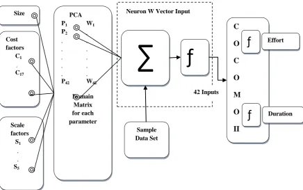
Refer Figure 1

Proposed system follows specific steps in which the flow is maintained. The details of each stage are mentioned below.

3.1

Input Actual Dataset Collected as Per

Project Specification

Size

It is essential part for software cost estimation. For predicting the size of the project function point estimation is better than SLOC. This method includes number of inputs, number of outputs, number of inquiries, number of logical files, number of interfaces by using this parameters we can find the projects complexity like simple, average, complex [7].

Table 1: Functional Units with weighting factors Functional Units Simple Avg Complex Total

User Inputs --×3 --×4 --×6 User Outputs --×4 --×5 --×7 User Queries --×3 --×4 --×6 Internal Logical

Files

--×7 --×10 --×15

External Interface Files

--×5 --×7 --×10

Total UFP (Unadjusted Function Point) =

Above functional units depends upon the rating values. Rating values having three levels: Simple, Average & Complex.

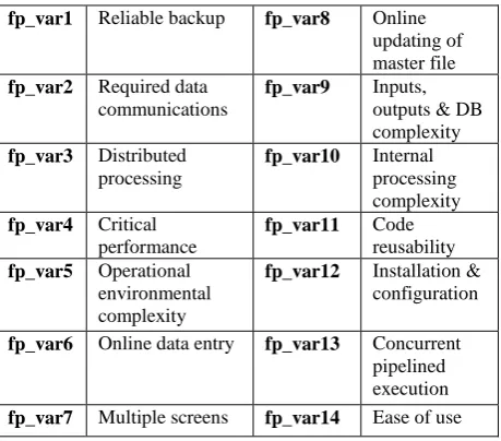
Table 2: Technical Complexity factors fp_var1 Reliable backup fp_var8 Online

updating of master file

fp_var2 Required data communications

fp_var9 Inputs, outputs & DB complexity

fp_var3 Distributed processing

fp_var10 Internal processing complexity

fp_var4 Critical performance

fp_var11 Code reusability

fp_var5 Operational environmental complexity

fp_var12 Installation & configuration

fp_var6 Online data entry fp_var13 Concurrent pipelined execution

fp_var7 Multiple screens fp_var14 Ease of use

In Table 2 each component can change from 0 to 5.

Calculate the Technical Complexity factor (TCF) using following equation:

𝑇𝐶𝐹 = 0.65 + 0.01( fp_var𝑖(i = 1 to 14)) 𝐹𝑃 = TCF ∗ UFP

𝑆𝐼𝑍𝐸 = Select language ∗ FP

Note: SIZE in KLOC

Cost factors

Boehm introduced a set of 17 cost drivers in the COCOMOII that adds accuracy to the COCOMO81. The cost drivers are grouped in four categories:-

Product factors: It is formulated with factors of product such as Required Software Reliability (RELY), Data Base Size (DATA), Product Complexity (CPLX), Developed for Reusability (RUSE) and Documentation Match to Life-Cycle Needs (DOCU).

Computer factors: It depends on Execution Time Constraint (TIME), Main Storage Constraint (STOR), and Platform Volatility (PVOL).

Figure 1: Proposed System Architecture Design for Software Cost Estimation.

(PCON), Application Experience (AEXP), Platform Experience (PEXP), Language and tool experience (LTEX).

Project factors: It depends upon project features such as Use of Software Tools (TOOL), Multisite Development (SITE) and Required Development Schedule (SCED). Table3 below shows the different cost factors with their rating values.

Table 3: Cost Factors

Factor VL L N H VH EH

(RELY) 0.75 0.88 1.00 1.15 1.40 - (DATA) - 0.94 1.00 1.08 1.16 - (CPLX) 0.70 0.85 1.00 1.15 1.30 1.65 (RUSE) - 0.89 1.00 1.16 1.34 1.56 (DOCU) 0.85 0.93 1.00 1.08 1.17 - TIME - - 1.00 1.11 1.30 1.66 (STOR) - - 1.00 1.06 1.21 1.56 (PVOL) - 0.87 1.00 1.15 1.30 - (ACAP) 1.5 1.22 1.00 0.83 0.67 - (PCAP) 1.37 1.16 1.00 0.87 0.74 - (PCON) 1.26 1.11 1.00 0.91 0.83 - (AEXP) 1.23 1.10 1.00 0.88 0.80 - (PEXP) 1.26 1.12 1.00 0.88 0.80 - (LTEX) 1.24 1.11 1.00 0.90 0.82 - (TOOL) 1.20 1.10 1.00 0.88 0.75 - (SITE) 1.24 1.10 1.00 0.92 0.85 0.79 (SCED) 1.23 1.08 1.00 1.04 1.10 -

Above cost factors depends upon the rating values corresponding to real number known as effort multipliers (EM). Rating values having six levels: Very low, Low, Nominal, High, Vey high, Extra high [19].

Scale factors

COCOMOII depends on the five scale factors such as Precedentedness (PREC), Development Flexibility (FLEX), Architecture / Risk Resolution (RESL), Team Cohesion (TEAM) and Process Maturity (PMAT).

Table 4: Scale Factors

Factor VL L N H VH EH

(PREC) 6.2 4.96 3.72 2.48 1.24 0 (FLEX) 5.07 4.05 3.04 2.03 1.01 0 (RESL) 7.07 5.62 4.24 2.83 1.41 0 (TEAM) 5.48 4.38 3.29 2.19 1.1 0 (PMAT) 7.8 6.24 4.68 3.12 1.56 0

3.2

Classification Using PCA

Why PCA is better than Fuzzy logic?

i. To find exact principal components rather than approximate like if the value is 0.99 consider it as 0.99 and not 1.00 by making it a round figure. ii. It allows us to identify the principal directions in

which the data varies with large variance [21]. Steps for calculating number of principal component are given below [2].

i. Calculate the correlation coefficient matrix ii. Calculate the eigenvalue of correlation coefficient

matrix.

iii. Determine the number of principal components.

42 Inputs Size

Cost factors C1 .

C17

Scale factors S1 .

.

S5

PCA P1 W1

P2 .

. .

. .

. .

. .

. .

P42 W42

Domain Matrix for each parameter

∑

Sample Data Set

ƒ

C

O

C

O

M

O

II

ƒ

The principal components will be determined based on following stages:

COCOMO sample data set -> quantify the data -> process missing data --> Calculate the correlation coefficient matrix -> Calculate the eigenvalue of correlation coefficient matrix -> Determine the number of principal components.

More important data in the project estimation is collected in the sample data set (COCOMO) which consists of many important factors for effort estimating such as software size, effort, productivity, development progress of project, project attributes, platform attributes, scale attribute, architecture and so on. Then quantify the data before processing the data. The sample data set should be preprocessed, because some data might get missed, in the mean time for calculating the eigenvalue we should calculate correlation coefficient matrix of input values and finally we should determine the number of principal components based on size, cost factors and scale factors as shown in figure 1.

3.3

Artificial Neural Network

Why we choose ANN?

Artificial Neural Network is used in cost estimation due to its ability to learn from previous data.

The three factors that define ANN are as follows:

i. The interconnection pattern between different layers of neurons.

ii. The learning process for updating the weights of the interconnections.

iii. The activation function that converts a neuron's weighted input to its output activation.

The nodes in the network are divided into input layer; associated with weights which contain information about the input signals and output layer which are going through the network to some nodes in hidden layer.

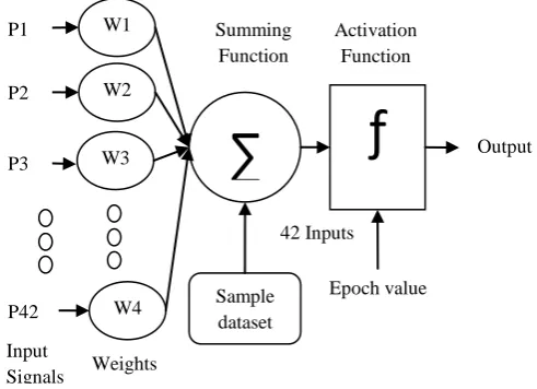
ANN Architecture:

Depending upon the architecture of the ANN it can be classified in two types namely; feed-forward ANN where the network has no loops and information moves in only one direction, i.e. forward from the input nodes then through the hidden nodes to the output nodes and the second is feed-back ANN where loops occurs in the network. An ANN can be a single-layer perception or a multi-layer perception. Single layer perception consists of a single layer of output nodes; the inputs neurons are connected directly to the outputs neurons via a series of weights, but in multi layer perception an additional layer of neurons are present between input and output layers which is called as hidden layer. Number of hidden layers can be added in an ANN depending upon the problem domain and accuracy expected. This paper has used multiple layers feed-forward ANN for simulation.

Figure 2: Architecture of Feed-forward neural network

A basic neural network consists of a number of inputs that are applied by some weights which are combined together to give an output. Different neural network learning algorithms are used such as Perceptron learning, Delta rule leaning, back propagation learning etc. We have used Delta rule learning algorithm to train the neural network and solve the different problems. Delta rule learning algorithm uses sigmoid activation function where each neuron has a continuous activation function instead of a threshold activation function. Following steps shows working of neural network:

Step1: The input layer receives input signal i.e. principal components from PCA and sends it to the hidden layer.

Step 2: It includes data training.

Training algorithm includes following steps:

i. Choose the training sample dataset and train it with principal components.

ii. Determine error in hidden layer but there is less chances of error because PCA provides exact eigenvalue.

iii. If error occurs then update the neural network weights.

iv. Repeat until the neural networks error is sufficiently small after an epoch is complete.

Step 3: Output layer sends size, effort multiplier and scale factor rating values to COCOMOII by using activation function as shown in figure 1.

3.4

COCOMOII

COCOMOII is the latest version of COCOMO.COCOMO81 dataset includes 63 historical projects and COCOMOII dataset includes 161 historical projects. The estimated effort in person-months (PM) for the COCOMOII is given as:

𝐸𝑓𝑓𝑜𝑟𝑡 = 𝐴 × 𝑆𝐼𝑍𝐸 𝐸_{× 𝐸𝑀}

𝑖 (1) 17

𝑖=1

𝑊ℎ𝑒𝑟𝑒 𝐸 = 𝐵 + 0.01 × 𝑆𝐹𝑗 5

𝑗 =1

𝐴 = 2.94, 𝐵 = 0.91 42 Inputs W1

W2

W3

W4 2 P1

P2

P3

P42

Weights

∑

Sample dataset

ƒ

Function

Activation Function

Output

Epoch value

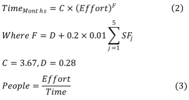
𝑇𝑖𝑚𝑒𝑀𝑜𝑛𝑡 ℎ𝑠= 𝐶 × 𝐸𝑓𝑓𝑜𝑟𝑡 𝐹 2

𝑊ℎ𝑒𝑟𝑒 𝐹 = 𝐷 + 0.2 × 0.01 𝑆𝐹𝑗 5

𝑗 =1

𝐶 = 3.67, 𝐷 = 0.28

𝑃𝑒𝑜𝑝𝑙𝑒 =𝐸𝑓𝑓𝑜𝑟𝑡

𝑇𝑖𝑚𝑒 (3)

COCOMOII uses function point size estimation method for calculating the size of the software and composes of 17 Effort multipliers and 5 scale factors (SF) as shown in Table 3, Table 4 [3].

𝐶𝑜𝑠𝑡 = 𝐸𝑓𝑓𝑜𝑟𝑡 × 𝑃𝑎𝑦𝑚𝑒𝑛𝑡𝑀𝑜𝑛𝑡 ℎ + 𝑂𝑡ℎ𝑒𝑟 𝑒𝑥𝑝𝑒𝑛𝑠𝑒𝑠 (4)

Other expenses means consider electricity charge, Maintenance of computer etc.

4.

POTENTIAL SIGNIFICANCE OF

THE PROPOSED MODEL

i. Support large domain space.

ii. Finding principal component than centre value. iii. Learning using standard database: It uses standard

rating values which is provided by Constructive Cost Model (COCOMO).

iv. Improving accuracy: PCA provides exact mean value due to this exact mean value accuracy of the model automatically increases.

v. Improving turnaround time.

vi. Very profound information is easily available.

5.

RESULTS AND DISCUSSION

Performance measure depends on following equation:

𝑀𝑅𝐸 = 𝐴𝑐𝑡𝑢𝑎𝑙 𝐸𝑓𝑓𝑜𝑟𝑡 − 𝐸𝑠𝑡𝑖𝑚𝑎𝑡𝑒𝑑 𝐸𝑓𝑓𝑜𝑟𝑡 _{𝐸𝑠𝑡𝑖𝑚𝑎𝑡𝑒𝑑 𝐸𝑓𝑓𝑜𝑟𝑡}

MRE (Magnitude of Relative Error)

Table 5: Comparison of Models Project Actual

Effort

COCOMO II

ANN Hybrid

1 670 846.83 819.44 778.33

2 360 507.17 487.89 457.69

3 70 126.51 117.17 102.69

4 18 39.36 35.10 27.71

5 72 82.49 75.60 64.40

Table 6: MRE Result Project MRE of

COCOMO II

MRE of ANN

MRE of Hybrid

1 0.26 0.22 0.16

2 0.40 0.35 0.27

3 0.80 0.67 0.46

4 1.18 0.95 0.53

5 0.14 0.05 0.10

Figure 3: Comparison of Estimated Vs Actual Effort

6.

CONCLUSION

There are large numbers of software available in the market to estimate cost of the software. The implications of the results are based on the COCOMO sample data set. The COCOMO repository consists of more than 161 projects collected from different countries around the world. In this proposed model, PCA and NN produces estimates that are more accurate than the ones provided by the same kind of algorithm without applying PCA and NN. Important result is that the proposed technology increases the correctness of the estimates without worsening the variability which improves the accuracy, turnaround time and performance of the system

7.

FUTURE SCOPE

Software development has become a crucial and important investment for many organizations. Now day’s Software engineering practitioners are becoming aware about accurately predicting the cost and quality of software product under development. The KPCA (Kernel Principal Component Analysis) model exhibits a significantly different

classification bias, a characteristic that makes it a valuable ensemble. The results confirm that accuracy is generally improved by the addition of the KPCA-based model.

8.

REFERENCES

[1] Anupama Kaushik, Ashish Chauhan, Deepak Mittal, Sachin Gupta. 2012.COCOMO Estimates Using Neural Networks I.J. Intelligent Systems and Applications, 2012, 9, 22-28 Published Online August 2012 in MECS [2] Bo Cheng, Xuejun Yu. 2012. The Selection of Agile

Development’s Effort Estimation Factors based on Principal Component Analysis. International Conference on Information and Computer Applications (ICICA 2012),IPCSIT vol. 24 IACSIT Press, Singapore 2012. [3] Vahid Khatibi, Dayang N.A.Jawawi. 2011. Software

Cost Estimation Methods: A Review, Vol. 2 No. 1 Journal of Emerging Trends in Computing and Information Science.CIS Journal.

[4] Attarzadeh I. Siew Hock Ow.2010. Improving the accuracy of software cost estimation model based on a new fuzzy logic model, World Applied science journal 8(2) 2010.

[5] Attarzadeh,I. Siew Hock Ow.2010. Proposing a New Software Cost Estimation Model Based on Artificial Neural Networks, IEEE International Conference on Computer Engineering and Technology (ICCET), Volume: 3, Page(s): V3-487 - V3-491 2010.

0 100 200 300 400 500 600 700 800 900

1 2 3 4 5

E

ff

o

rt

Project

[6] Khaled Hamdan 2010. Practical Software Project Total Cost Estimation Methods. IEEE 2010

[7] Sikka, G., A. Kaur, et al. 2010. Estimating function points: Using machine learning and regression models. Education Technology and Computer (ICETC), 2nd International Conference on, 2010.

[8] Justin Wong Danny Ho Luiz Fernando Capretz 2009. An Investigation of Using Neuro-Fuzzy with Software Size Estimation. IEEE ICSE’09 Workshop May 16, 2009, Vancouver, Canada

[9] Chiu, N.H., Huang, S.J. 2007. The adjusted analogy-based software effort estimation analogy-based on similarity distances, Journal of Systems and Software 80 (4), 628– 640.2007

[10]Y. F. Li, M. Xie, T. N. Goh. 2007. A Study of Genetic Algorithm for Project Selection for Analogy Based Software Cost Estimation. IEEE 2007.

[11]Marcio R., Silvia Regina. 2006. Software Effort Estimation Based on Use Cases. IEEE 2006.

[12]Jørgensen, M. 2005. Practical guidelines for expert-judgment-based software effort estimation, IEEE Software, 22(3), 57-63. doi:10.1109/MS. 73, 2005.

[13]Xishi Huang, Luiz F. Capretz, Jing Ren 2003. A Neuro-Fuzzy Model for Software Cost Estimation. IEEE 2003. [14]Musilek A.2002. On the Sensitivity of COCOMO II

Software Cost Estimation Model, IEEE 2002.

[15]Shepperd M.1997. Estimating Software Project Effort Using Analogies IEEE NOV. 1997.

[16]K. Srinivasan and D. Fisher.1995. Machine Learning Approaches to Estimating Software Development Effort, IEEE Transactions on Software Engineering, 21 (2), 1995.

[17]Kemerer, C. 1987. An empirical validation of software cost estimation models, Communications of the ACM, 30(5), 416-429. doi: 10.1145/22899. 22906, 1987. [18]Albrecht. A.J. and J. E. Gaffney.1983. Software function,

source lines of codes, and development effort prediction: a software science validation, IEEE Trans Software Eng. SE, pp.639-648, 1983.

[19]Boehm B. W.1981. Software Engineering Economics, Englewood Cliffs, NJ, Prentice-Hall, 1981.

[20]Max Welling Kernel Principal Components Analysis. [21]dr inż. Małgorzata Syczewska, dr inż. Piotr Wąsiewicz.