Local likelihood estimation of truncated regression and its partial derivatives: theory and application

Munich Personal RePEc Archive

Local likelihood estimation of truncated

regression and its partial derivatives:

theory and application

Park, Byeong and Simar, Leopold and Zelenyuk, Valentin

Institut De Statistique, Universite Catholique de Louvain

19 March 2006

Online at

https://mpra.ub.uni-muenchen.de/34686/

I N S T I T U T

D E

S T A T I S T I Q U E

UNIVERSIT´E CATHOLIQUE DE LOUVAIN

D I S C U S S I O N

P

A

P

E

R

0606

LOCAL LIKELIHOOD ESTIMATION

OF TRUNCATED REGRESSION

AND ITS PARTIAL DERIVATIVES:

THEORY AND APPLICATION

B.U. PARK, L. SIMAR and V. ZELENYUK

Local Likelihood Estimation of Truncated Regression

and Its Partial Derivatives: Theory and Application

Byeong U. Park

Department of Statistics

Seoul National University

L´eopold Simar

Institut de Statistique

Universit´e Catholique de Louvain

Valentin Zelenyuk

KEI - Kyiv Economics Institute

UPEG/EERC

National University, Kyiv-Mohyla Academy

March 19, 2006

Abstract

In this paper we propose a very flexible estimator in the context of truncated regression that does not require parametric assumptions. To do this, we adapt the theory of local maximum likelihood estimation. We provide the asymptotic results and illustrate the performance of our estimator on simulated and real data sets. Our estimator performs as good as the fully parametric estimator when the assumptions for the latter hold, but as expected, much better when they do not (provided that the curse of dimensionality problem is not the issue). Overall, our estimator exhibits a fair degree of robustness to various deviations from linearity in the regression equation and also to deviations from the specification of the error term. So the approach shall prove to be very useful in practical applications, where the parametric form of the regression or of the distribution is rarely known.

Key words : Nonparametric Truncated Regression, Local Likelihood.

JELClassification: C14, C24

∗_{Research of B. U. Park was supported by the Korea Research Foundation Grant funded by the Korean}

Government (MOEHRD) (KRF-2005-070-C00021)

†_{Research support from the “Interuniversity Attraction Pole”, Phase V (No. P5/24) from the Belgian}

1

Introduction

In this paper we consider the problem of estimating a regression model where the support of the continuous dependent variable is bounded at a known constant at one end and when many of the observations are observed near this bound. This is a common case when the dependent variable is an economic index measured within some range. One example in the recent econometric literature of such context is the analysis of how some economic variables determine the level of the Debreu (1951)-Farrell (1957) type efficiency score (bounded be-tween 0 and 1 or, taking its inverse, bebe-tween 1 and infinity, with many values concentrated near unity). A similar example can be drawn for the applied consumer analysis, where the so-called Luenberger (1994)-Chamberset al. (1996) shortage/benefit or directional distance function (bounded between zero and infinity, with most values being close to zero) can be used to analyze consumer benefits. An appropriate way of handling such problems is to use the truncated regressionapproach (see Simar and Wilson, 2006, for a parametric case).

The traditional truncated regression approach is based on using fully specified parametric model, where both the functional form of the relationship between the dependent and ex-planatory variables and the functional form of the distribution of the error term is specified. A natural estimator therefore is based on the maximum likelihood principle. An obvious drawback of such approach is the reliability of parametric assumptions and vulnerability to deviations from them. Indeed, a mistake in specifying a parametric form of the regression equation or of the distribution of the error may lead to inconsistent estimation. The goal of our study is to propose a more flexible estimator for the context of truncated regression that does not require such parametric assumptions.

of-fered by the local likelihood methods help circumventing these problems substantially, as we demonstrate with some simulated examples.

The theoretical foundation for our paper is based on a recent paper of Kumbhakar et al. (2006) who extended and generalized the approach suggested by Fan et al. (1996). In our work we make further extension. First, we adapt the theory to the truncated regression case. Second, and most importantly, we provide asymptotic results for the derivatives of regression function, which is the main focus of our paper, because many economic studies are concerned with the marginal effects of some variables on others. Third, our treatment includes both the cases where the shape parameter of the error distribution is an unknown constant, and where it is an unknown smooth function. In the former case, our estimator of the shape parameter achieves root-n consistency, and so does not suffer from the curse of dimensionality. Fourth, we show that fitting a lower order polynomial for the shape param-eter may jeopardize the estimator of the regression function. This justifies consideration of higher-order local polynomial fit for the shape parameter even if one is mainly interested in estimating the regression function and its derivatives.

Our paper is structured as follows. In Section 2, we describe the local likelihood trun-cated regression methods. In Section 3, we present the asymptotic theory of local likelihood adapted to the truncated regression case of our type. In Section 4, we illustrate the perfor-mance of our estimator on several simulated data sets, considering different scenarios about regression equation and the error. In Section 5, we illustrate our estimator for a real data set. Section 6 concludes and Section 7 gives the regularity conditions for obtaining our results and outlines the proof of the theorems.

2

Local Polynomial Estimation

2.1

Constant Shape Parameter Case

We observe a set of i.i.d. random variables (Xi, Yi) for i = 1, . . . , n with Xi ∈ IRd and

Yi ∈IR, where

Yi =f(Xi) +εi ≥c

for some unknown functionf and a known positive constantc. In this model,ε, conditionally on X = x, has a continuous distribution G(·, τ) truncated below c−f(x), where τ is an unknown shape parameter that is assumed to be a constant. In other words, the conditional density ofY given X =x equals

ϕ(y, f(x), τ)_≡ gε(y−f(x), τ)

where gε(ε, τ) = ∂G(ε, τ)/∂ε. We assume that G is known. Our main interest here is

esti-mation of the functionf and its derivatives. Below we describe local polynomial estimation of f in a general setting of multivariate X.

Note that all the results obtained in this paper could be easily adapted to the case where the dependent variable is truncated at both sides : c1 _≤ Yi ≤ c2. This would only change

the definition of ϕ(y, f(x), τ), the conditional density of Y given X =x.

Define ℓ= logϕ. Then, the conditional log-likelihood equals Pn_i=1ℓ(Yi, f(Xi), τ). Let x

be a point at which one wants to estimate the values of the function f and its derivatives. A local conditional log-likelihood is obtained by replacingf in the conditional log-likelihood by its pth order polynomial approximation in a neighborhood of x and putting the weight

Kh(Xi−x) for each observation (Xi, Yi), whereKh(u) =h−dK(h−1u),K is ad-variate kernel

function, typically a symmetric density function defined on IRd, and h is a positive scalar, called the bandwidth. Precisely, it is given by

Ln(θ0, θ1, . . . , θr(p)−1, τ;x)

=

n X

i=1

ℓ Yi, θ0 +θ1(Xi1−x1) +· · ·+θr(p)−1(Xid−xd)p, τ

Kh(Xi−x),

wherer(p)₋1 is the total number of partial derivatives up to orderp, i.e.,r(p) = Pp_j=0 j+_d−d−₁1

. Here and below,Xi ≡(Xi1, . . . , Xid)T andx≡(x1, . . . , xd)T. Thepth order local polynomial

estimators offand its derivatives atxare obtained by maximizingLn(θ0, θ1, . . . , θr(p)−1, τ;x).

For example, ˆf(x) = ˆθ0(x) and the estimator off′_{(x)≡[∂f(x)/∂x1, . . . , ∂f(x)/∂x}

d]T is given

by ˆf′_{(x) = [ˆθ1(x), . . . ,θ}ˆ

d(x)]T, where

ˆ

θ0(x),θ1ˆ(x), . . . ,θˆr(p)−1(x),τ˜(x)

= arg max

θ0,...,θr(p)−1,τ

Ln(θ0, θ1, . . . , θr(p)−1, τ;x). (2.1)

The estimator ˜τ is obtained locally in the above local polynomial estimation procedure, and thus it depends onx. It can be improved by maximizing the full likelihood withf being replaced by its estimator ˆf, i.e, a better estimator is given by

ˆ

τ = arg max

τ n X

i=1

ℓ(Yi,fˆ(Xi), τ). (2.2)

One may further update the estimators ˆθj(x) by maximizingLn(θ0, θ1, . . . , θr(p)−1,ˆτ;x) where

τ on the right hand side of (2.1) is replaced by ˆτ, now with respect toθ0, θ1, . . . , θr(p)−1 only.

2.2

Functional Shape Parameter Case

parameter is not a constant, fitting a local constant forτ as in the previous subsection pro-duced poor estimates off and its derivatives. This motivated us to consider fitting a higher order local polynomial for the functionτ. As illustrated in the simulation study reported in Section 4 below, fitting a local linear for τ worked particularly well.

When the shape parameter is a function, the conditional log-likelihood is given by

Pn

i=1ℓ(Yi, f(Xi), τ(Xi)), whereℓ(y, ν, ω) = log [gε(y−ν, ω)I(y≥c)/{1−G(c−ν, ω)}]. We

fit aqth order local polynomial for the functionτ, i.e., we take the following local conditional log-likelihood:

Ln(θ0, . . . , θr(p)−1, τ0, . . . , τr(q)−1;x)

=

n X

i=1

ℓ Yi, θ0+θ1(Xi1−x1) +· · ·+θr(p)−1(Xid−xd)p,

τ0+τ1(Xi1−x1) +· · ·+τr(q)−1(Xid−xd)q

Kh(Xi−x).

The local polynomial estimators off, τ and their derivatives atxare obtained by maximizing

Ln(θ0, θ1, . . . , θr(p)−1, τ0, . . . , τr(q)−1;x), i.e.,

ˆ

θ0(x), . . . ,θˆr(p)−1(x),τ0ˆ(x), . . . ,τˆr(q)−1(x)

(2.3)

= arg max

θ0,...,θr(p)−1,τ0,...,τr(q)−1

Ln(θ0, θ1, . . . , θr(p)−1, τ0, . . . , τr(q)−1;x).

3

Theoretical Properties

Here, we provide the asymptotic distributions of the estimator defined at (2.1) and (2.3). The theory we present here does not rely on the assumption that the log-likelihood function

ℓ(y, ν, ω) as a function of (ν, ω) is globally concave for each y. The latter assumption is usually imposed for methods based on the local likelihood approach, see Fan et al. (1995) or Carroll et al. (1997), for example.

3.1

Constant Shape Parameter Case

The results we present below is closely related to those of Kumbhakaret al. (2006). However, the latter treated only the local linear estimator for multivariateX in some different setting. We give more general results for the local polynomial estimators defined at (2.1).

For 0_≤i, j _≤2 with i+j = 1,2, let

For ad-vectoru, letzp(u) = (1, u1, . . . , up_d)T, anr(p)-vector. For a vectora≡ a0, . . . , ar(p)−1

T

and a scalarb, define Q(a, b) = [Q1(a, b)T_{, Q2(a, b)]}T _where

Q1(a, b) =

Z

Ehℓ10 Y, f(x) +a0+a1u1+· · ·+ar(p)−1upd, τ +b

X =x

i

zp(u)K(u)du,

Q2(a, b) =

Z

Ehℓ01 Y, f(x) +a0+a1u1+· · ·+ar(p)−1upd, τ +b

X =x i

K(u)du.

Our results require that the system of equations Q(a, b) = 0 has a unique solution (aT_{, b)}T_.

Let

ρij(x) =−E[ℓij(Y, f(x), τ)|X =x].

It can be shown that ifρ20(x)>0,ρ20(x)ρ02(x)−ρ11(x)2 _{>0, and K ≥0 is supported on a}

set which contains ad-dimensional open rectangle, then Qn(a, b) = 0 has a unique solution.

As in Kumbhakaret al. (2006), the uniqueness of the solution plays an important role for a stochastic expansion of the estimators.

The presentation needs some careful notations to treat the multivariateX and the higher order approximating polynomial. First, for ad-tuplek _≡(k1, . . . , kd) and ad-vectorx, write

k! =k1!× · · · ×kd!, |k|= d X

i=1

ki, xk =xk11 × · · · ×x

kd

d .

For a functionη defined on IRd, write

∇kη

(x) = ∂

|k|_η(x)

∂xk1

1 · · ·∂x

kd

d

.

Let mj = j+_d−d−₁1

for j ≥ 0. Arrange mj number of d-tuples k with |k| = j in a

counter-lexicographical order: put (j,0, . . . ,0) first and (0,0, . . . , j) last. Let ξj denote the function

which maps an integer s for 1 ≤ s ≤ mj to the one located at the sth position in the

ar-rangement of thed-tuples of sizej. For example, ξj(1) = (j,0, . . . ,0). Let µk = R

uk_K(u)du

for a d-tuple k. For j, l _≥ 0 denote by Njl the mj ×ml matrix whose (s, t)th entry equals

µξj(s)+ξl(t). Define r(p)×mj matrices N

(p)

j = N0Tj, . . . , NpjT T

for j = 0, . . . , p+ 1, and a

r(p)_×r(p) matrix N(p,p) _{= N}(p)

0 , . . . , N (p)

p

. Likewise, define Mjl, Mj(p) and a r(p)×r(p)

matrixM(p,p) _{by replacingµ}

k in the definitions ofNjl, Nj(p) andN(p,p)byκk = R

uk_K2_(u)du.

Now we define [r(p) + 1]_×[r(p) + 1] matrices

D(x) =

"

N(p,p)ρ20(x) N0(p)ρ11(x) N₀(p)Tρ11(x) N00ρ02(x)

#

, V(x) =

"

M(p,p)v20(x) M0(p)v11(x) M₀(p)Tv11(x) M00v02(x)

#

,

wherev20(x) = E[ℓ2

andK ≥0 is supported on a set which contains ad-dimensional open rectangle, thenD(x) is positive definite. Under the latter condition on K, the matrixV(x) is also positive definite unless there exists a nonzero constant c such that ℓ10(Y, f(x), τ) = c ℓ01(Y, f(x), τ) with

probability one, conditionally onX=x. Let _D(p,p)_{(x) be the r(p)×r(p) upper-left block of}

D(x) =D(x)−1_.

To translate each of ˆθi(x) defined at (2.1) to an estimator of f(x) or its derivatives, we

consider blocks of sizemj, j = 0, . . . , p, in the vector of ˆθi(x). Write ˆθ(0)(x) = ˆθ0(x), and let

ˆ

θ(j)_{(x) for j ≥1 be the jth block of size m}

j defined by

ˆ

θ(j)(x) = [ˆθr(j−1)(x), . . . ,θˆr(j)−1(x)]T.

Thus, ˆθ(1)_{(x) =}h_θ1ˆ_{(x), . . . ,θ}ˆ

d(x) iT

, and so on. Furthermore,

ˆ

θ(x)≡[ˆθ0(x), . . . ,θˆr(p)−1(x)]T = [ˆθ(0)(x),θˆ(1)T(x), . . . ,θˆ(p)T(x)]T.

Define Ej(p) by E

(p)T j =

Omj×r(j−1), Imj, Omj×(r(p)−r(j))

, where Or×s denote the r×s zero

matrix, and Ir is the r-dimensional identity matrix. For j = 0, . . . , p, Ej(p) is a r(p)×mj

matrix which maps the whole ˆθ(x) to ˆθ(j)_{(x) by}

ˆ

θ(j)_{(x) =E}(p)T j θˆ(x).

Let θ(j)(x) be the mj-vector of all the jth partial derivatives of f(x) divided by the

corre-sponding factorials, arranged in the counter-lexicographical order, i.e.,

θ(j)_{(x) = [∇}ξj(1)_f(x)/ξ

j(1)!, . . . ,∇ξj(mj)f(x)/ξj(mj)!]T. (3.1)

Then, ˆθ(j)_{(x) is the local polynomial estimator of θ}(j)_(x).

Letg(x) denote the marginal density function ofX. Let_Uj,f(p:0)be the [r(p)+1]_×mj matrix

obtained by adding the row vectorO1×mj at the bottom ofE

(p)

j , i.e.,U

(p:0)T j,f = (E

(p)T

j , Omj×1).

Also, write _U0(p_,τ:0) for the [r(p) + 1]-dimensional unit vector (0,0, . . . ,0,1)T_{. We obtain the}

following theorem.

Theorem 3.1. Under the assumptions (A1)–(A9) given in Section 7, it follows that for each j = 0, . . . , p

√

nh2j+dh_θˆ(j)_(x)−θ(j)_(x)−hp−j+1_ρ20(x)E(p)T

j D(p,p)(x)N

(p)

p+1θ(p+1)(x) +o(hp−j+1)

i

d

−→ Nmj

h

0,Uj,f(p:0)TD(x)V(x)D(x)U

(p:0)

j,f /g(x) i

,

whereNrdenotes anr-variate normal distribution. Forτ˜(x), denoting the(r+2)-dimensional

unit vector (0,0, . . . ,0,1)T _{by e}

r+2, we have

√

nhd_{(˜τ(x)−τ)−→ N}d

1

h

0,U0(p,τ:0)TD(x)V(x)D(x)U

(p:0) 0,τ /g(x)

i

The theorem tells that thepth order local polynomial estimators of thejth partial deriva-tives converge to the true values at the rate hp−j+1 _+n−1/2_h−d/2−j_{. In fact, if all the odd}

order moments ofK vanish, i.e., R

uk_{K(u)du= 0 for all d-tuples k with |k|= 1,3, . . . , and}

p₋j is even, then it can be shown that the leading bias term of order hp−j+1 _{is zero. In this}

case, ifθ(p+2)_{(x) as defined at (3.1) exists and is continuous, then the bias is of orderh}p−j+2_.

The theorem also gives the rate of the convergence of ˜τ(x) as an estimator of the constant

τ, which is n−1/2_h−d/2_{. Note that it does not have a bias term since the true value τ is a}

constant whose derivatives are all zero. However, the raten−1/2_h−d/2 _{is inferior to the usual} n−1/2 _{for the parametric components. This is because one only takes a fraction of data of}

size nhd _{in the local fitting procedure at (2.1). The estimator defined at (2.2), which uses}

the full likelihood with f being replaced by its estimator ˆf = ˆθ0, may be shown to achieve

the n−1/2 _{rate, see Carroll et al. (1997) for a proof of this kind in a different setting.}

3.2

Functional Shape Parameter Case

In this subsection we present the asymptotic distributions of ˆθj(x) for j = 0,1, . . . , r, and

ˆ

τj(x) for j = 0,1, . . . , s, defined at (2.3). We slightly modify the definitions of the terms

that are used in Subsection 3.1, whenever necessary, and introduce more to treat the case where the shape parameter τ is an unknown function.

With slight abuse of notation, we continue to use the same notation ρij and vij, which

are now defined as

ρij(x) = −E[ℓij(Y, f(x), τ(x))|X =x],

v20(x) = E

ℓ210(Y, f(x), τ(x))|X =x

, v02(x) = E

ℓ2₀₁(Y, f(x), τ(x))|X =x

,

v11(x) = E[ℓ10(Y, f(x), τ(x))ℓ01(Y, f(x), τ(x))_|X =x].

Forr(p)-vectors a _≡ (a0, . . . , ar(p)−1)T and b ≡ (b0, . . . , br(p)−1)T, we also modify the

defini-tions of Qj(a, b) as

Q1(a, b) =

Z

Ehℓ10 Y, f(x) +a0+a1u1+· · ·+ar(p)−1upd,

τ(x) +b0+b1u1+· · ·+br(q)−1uqd

X =x

i

zp(u)K(u)du,

Q2(a, b) =

Z

Ehℓ01 Y, f(x) +a0+a1u1+_{· · ·}+ar(p)−1upd,

τ(x) +b0+b1u1+_{· · ·}+br(q)−1uq_d

X =x

i

zq(u)K(u)du.

a set which contains ad-dimensional open rectangle, then the system of equationsQ1(a, b) = 0 andQ2(a, b) = 0 has the unique solution.

To state an analogue of Theorem 3.1, we need further notation. Define an r(p)_×r(q) matrix N(p,q) _{= N}(p)

0 , . . . , N (p)

q . Also, define N(q,p) = N₀(q), . . . , Np(q) and N(q,q) =

N₀(q), . . . , Nq(q), which are r(q)× r(p) and r(q)× r(q), respectively, matrices. Likewise,

define M(p,q)_{, M}(q,p) _{and M}(q,q) _{with µ}

k being replaced by κk = R

uk_K2_{(u)du. With these}

matrices, definitions of D(x) andV(x) are modified as

D(x) =

N(p,p)_{ρ20(x) N}(p,q)_ρ11(x) N(q,p)_ρ

11(x) N(q,q)ρ02(x)

, V(x) =

M(p,p)_{v20(x) M}(p,q)_v11(x) M(q,p)_v

11(x) M(q,q)v02(x)

.

These are [r(p) +r(q)]×[r(p) +r(q)] matrices.

As in Subsection 3.1, letD(p,p)_{(x) be the r(p)×r(p) upper-left block of D(x) = D(x)}−1_.

LetD(p,q)_{(x) be ther(p)×r(q) upper-right block,D}(q,p)_{(x) be ther(q)×r(p) lower-left block,}

and_D(q,q)_{(x) be the r(q)×r(q) lower-right block of D(x). Defineτ}(j)_{(x) in the same way as} θ(j)_{(x) with f replaced byτ in (3.1). Also, define}

ˆ

τ(j)(x) =_Ej(q)Tτˆ(x).

To express the biases of the estimators, define

B1,f(x) = ρ20(x)D(p,p)Np(p+1)θ(p+1)(x) +ρ11(x)D(p,q)(x)N (q)

p+1θ(p+1)(x), B2,f(x) = ρ11(x)D(p,p)Nq(p+1)τ(q+1)(x) +ρ02(x)D(p,q)(x)Nq(q+1) τ(q+1)(x), B1,τ(x) = ρ20(x)D(q,p)Np(p+1)θ(p+1)(x) +ρ11(x)D(q,q)(x)N

(q)

p+1θ(p+1)(x), B2,τ(x) = ρ11(x)D(q,p)Nq(p+1)τ(q+1)(x) +ρ02(x)D(q,q)(x)N

(q)

q+1τ(q+1)(x).

Finally, extending the definition of _Uj,f(p:0) in Subsection 3.1, let _Uj,f(p:q) be the [r(p) +

r(q)]×mj matrix obtained by adding the zero matrix Or(q)×mj at the bottom of E

(p)

j , i.e.,

Uj,f(p:q)T = (E

(p)T

j , Omj×r(q)). Also, letU

(p:q)

j,τ be the [r(p)+r(q)]×mj matrix obtained by adding

the zero matrix Or(p)×mj at the top of E

(q)

j , i.e., U

(p:q)T

j,τ = (Omj×r(p),E

(q)T

j ). We obtain the

following theorem.

Theorem 3.2. Under the assumptions (B1)–(B9) given in Section 7, it follows that for each j = 0, . . . , p

√

nh2j+dh_θˆ(j)_(x)−θ(j)_{(x)− E}(p)T

j (B1,fhp−j+1+B2,fhq−j+1) +o(hp−j+1+hq−j+1) i

d

−→ Nmj

h

0,Uj,f(p:q)TD(x)V(x)D(x)U

(p:q)

j,f /g(x) i

,

where Nr denotes an r-variate normal distribution. Also, for each j = 0, . . . , q

√

nh2j+dh_τˆ(j)_(x)−τ(j)_{(x)− E}(q)T

j (B1,τhp−j+1+B2,τhq−j+1) +o(hp−j+1+hq−j+1) i

d

−→ Nmj

h

0,Uj,τ(p:q)TD(x)V(x)D(x)U

(p:q)

j,τ /g(x) i

The theorem tells that both ˆθ(j) _{and ˆτ}(j) _{have the same order of bias even if one fits}

locally polynomials of different degrees forf and τ. The leading biases for ˆθ(j) _{and ˆτ}(j) _are

of the same order h(p∧q)−j+1_{, where p∧q = p if p ≤ q and p∧ q = q otherwise. Thus,}

the smaller of p and q determines the order of the bias for both ˆθ(j) _{and ˆτ}(j)_{. This means}

that fitting a lower order polynomial forτ may jeopardize the estimator off. This is a new theoretical finding. It explains the failure of the local constant fit for τ in our preliminary experiment, and justifies consideration of higher-order local polynomial fit forτ even if one is interested in estimating the functionf and its derivatives.

Here again, as discussed in Subsection 3.1, if all the odd moments of K vanish and (p∧q)−j is even, then the leading bias terms of ˆθ(j) _{and ˆτ}(j) _{are of orderh}(p∧q)−j+2 _provided

that θ((p∧q)+2)_{(x) andτ}((p∧q)+2)_{(x) exist and are continuous.}

4

Simulation Results

While constructing scenarios we had in mind a dependent variable bounded between 1 and infinity, with distribution skewed towards the unity bound, with most observations falling in between 1 and 2. Intuitively, this would be an index (e.g., the Debreu-Farrell efficiency index), whose reciprocal is then bounded between 0 and 100%, and most of which are between 50% and 100%. This is adequate to, for example, what many empirical studies report about production efficiencies of firms or countries (e.g., see Kumar and Russell, 2002, Zelenyuk and Zheka, 2006, etc. . . ). Such scenarios, with relatively small variation in the dependent variable and most of which being near the bound, are especially difficult to handle and so would be a good assessment experiment for our estimator.

In all the applications below, local linear fit was used for the shape parameter τ and we will compare the local linear and local quadratic fit for the regression function f. We used the Gaussian kernel and the bandwidth was determined by cross validation in the lines of

e.g. Kumbhakar et al. (2006).

We first consider the univariate case. This exercise is useful for visually observing the scenario and performance of our estimator relative to the plot of the true model and its traditional, fully parametric estimator. So our true model would be

Yi =f(Xi) +εi, i= 1, . . . , n, (4.1)

whereεi∼ N1 0, σε2(Xi)

, with εi ≥1−f(Xi).

4.1

Example 1. Linear Model with Homoskedasticity

In this scenario we assume homoskedastic variance before truncation, i.e., σε(Xi) = σ. So

we mean here that the shape parameter of the error term is homoskedastic whereas, after truncation the model obviously is heteroskedastic, because the variance would depend on the truncation point (1−f(Xi)). In addition, we assume also that the regression equation

is linear:

f(Xi) =β0 +β1Xi (4.2)

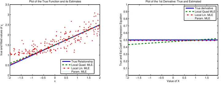
In this case, the traditional truncated regression model with linear regression function, and with homoskedactic shape parameter (before truncation) would be based on fully parametric maximum likelihood methods and would provide efficient estimators of the parameters. This is the approach studied in Simar and Wilson (2006). The goal of doing this experiment is to investigate how much do we lose (in a univariate case) by using our flexible approach and by not imposing the true parametric structure globally. Figure 1 visualizes this scenario and the estimation results for σ = 0.3, β0 = 1.5, β1 = 0.5. The Xi were generated according a

uniformU(₋2,2) and the sample sizen = 200.

−2 −1.5 −1 −0.5 0 0.5 1 1.5 2 0

0.5 1 1.5 2 2.5 3 3.5

x

true and fitted values of y

i

Plot of the True Function and its Estimates

True Relationship Local Quad. MLE. Local Lin. MLE Param. MLE

−2 −1.5 −1 −0.5 0 0.5 1 1.5 2 0

0.1 0.2 0.3 0.4 0.5 0.6 0.7 0.8 0.9 1

Plot of the 1st Derivative: True and Estimated

Value of X

True and Est.Coeff.of Regression Equation

True derivative Local Quad MLE Local Lin. MLE Param. MLE

Figure 1: Example 1: linear model and homoskedastic shape parameter. Left panel is the model and right panel is the derivative.

Left panel of Figure 1 shows the plot of the true function (solid line) we want to estimate and the fit of three estimators: parametric ML estimator (dotted line) and local linear like-lihood estimator (dash-dotted line) and local quadratic likelike-lihood estimator (dashed curve). We see that all the estimators give a very good fit virtually indistinguishable from each other and from the true function. (One might also notice that the quadratic fit has just a bit of curvature.)

give fairly good fit of derivatives as well. Note that the local linear likelihood estimator sug-gests that the true derivative is constant (as it is in reality). The local quadratic likelihood estimator suggests that the true derivative is slightly diminishing, which corresponds to a slight curvature we observed in the left panel of Figure 1. This should not be surprising: the linear approximation in the likelihood is the best approximation in this case. In practice, however, one can hardly know what the true parametric form of the regression equation is, so taking quadratic approximation is likely to give a better fit, as we will see from other examples where non-linearity or even linearity but with heteroskedasticity for the shape pa-rameter is present in the true model. Overall, for the univariate case, both linear and the quadratic local likelihood estimators perform very well relative to the truth and virtually as good as when we know and use the appropriate parametric assumptions.

4.2

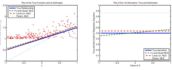
Example 2. Linear Model with Heteroskedasticity

In this scenario we assume heteroskedastic of the shape parameter before truncation, i.e.,

σε(Xi) now depends onx. Several diffrent scenarios have been tried here providing

qualita-tively the same kind of results. For saving space we present here only two interesting cases for the practitian.

• Case a_{. The more x forces Y to be closer to the bound the larger it makes σε(Xi).} This results in a lot of observations appearing very near the bound. (Figure 2 visualizes this scenario and the estimation results forσε(Xi) = (6−Xi)/10 with as aboveβ0 = 1.5, β1 = 0.5.

HereXi ∼U(−4,4) andn = 200.

• Case b_{. The more x forces Y to be away from the bound the larger it makes σε(Xi).} This results in a lot of observations appearing very near the bound. (Figure 3 visualizes this scenario and the estimation results forσε(Xi) = 0.2

√

Xi+ 3 with as aboveβ0 = 1.5, β1 = 0.5.

−4 −3 −2 −1 0 1 2 3 4 −0.5 0 0.5 1 1.5 2 2.5 3 3.5 4 x

true and fitted values of y

i

Plot of the True Function and its Estimates

True Relationship Local Quad. MLE. Local Lin. MLE Param. MLE

−1 −0.5 0 0.5 1

0 0.1 0.2 0.3 0.4 0.5 0.6 0.7 0.8 0.9 1

Plot of the 1st Derivative: True and Estimated

Value of X

True and Est.Coeff.of Regression Equation

True derivative Local Quad MLE Local Lin. MLE Param. MLE

Figure 2: Example 2, casea: linear model and heteroskedastic shape parameter. Left panel is the model and right panel is the derivative.

−1 −0.5 0 0.5 1

0 0.5 1 1.5 2 2.5 x

true and fitted values of y

i

Plot of the True Function and its Estimates True Relationship

Local Quad. MLE. Local Lin. MLE Param. MLE

−1 −0.5 0 0.5 1

0 0.1 0.2 0.3 0.4 0.5 0.6 0.7 0.8 0.9 1

Plot of the 1st Derivative: True and Estimated

Value of X

True and Est.Coeff.of Regression Equation

True derivative Local Quad MLE Local Lin. MLE Param. MLE

Figure 3: Example 2, case b: linear model and heteroskedastic shape parameter. Left panel is the model and right panel is the derivative.

Intuitively, Case asuggests that the explanatory variable is negatively affecting the level (indicated by the first moment) of dependent variable, but increases the risk (indicated by the variance) causing it being further away from the bound. On the other hand, Case b

suggests that the explanatory variable is negatively affecting the level of dependent variable and reduces the random risk. For example, in a production context, x can be number of employees: the more employees the greater is the principle-agent problem and the more human-driven mistakes can cause inefficiency in production process and so on.

is present, the fully parametric MLE that we used in the previous example performs poorly. This is because it does not take into account the form of heteroskedasticity, which is usually unknown in practice. On the other hand, both the linear and the quadratic local likelihood estimators capture the heteroskedasticity nature of the model and perform very well for the fit of the model and for the derivative. In this sense, our estimators should be very useful even when the regression model is linear but the form of heteroskedasticity is not known.

Note that in our simulation scenarios we do not restrict f(X) to be bounded or to have any particular shape. However, for modeling some particular phenomena, f(X) might be required to be above the threshold and so, for example, the linear model would be inappropriate there. For instance, the true f(X) might be a non-linear that asymptotes the threshold or makes a U-shape or has some periodicity, etc., but what exactly the form should be is hardly known in practice and so a non-parametric estimator is very desired. It might also be unknown if f(X) needs to be restricted or not. In all these cases, imposing particular form of f(X) in parametric ML estimation might lead to erroneous results and conclusions. The problem might be even more complicated if the shape parameter of the distribution is not a constant. Remarkably, without knowing anything aboutf(X) and the shape parameter, our non-parametric estimator is capable of recognizing, from the data, what shall be attributed to the curvature off(X) and what shall be understood as a curvature of the shape parameter, as we illustrate with further simulations and with the empirical illustration below.

4.3

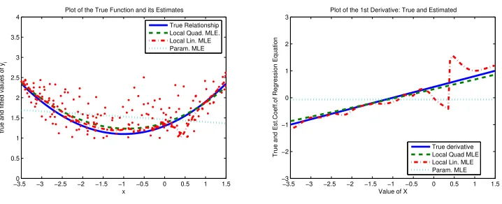
Example 3. Quadratic Model with Heteroskedasticity

In this scenario we assume the same true model as before but with an additional quadratic term β2x2

2 in model (4.2). We also assume heteroskedastic shape parameter, i.e., σε(Xi)

depends onx(we also investigate a scenario with homoskedastic shape parameter, providing very good results, but to save space we only present the more challenging case here). The goal of the exercise is to see if our estimators perform well in this non-linear case, complicated by heteroskedasticity. Figure 4 presents a typical estimation results, where σε(Xi) = 0.5−

0.05(Xi+ 1)2 with β0 = 1.3, β1 = 0.4 andβ2 = 0.2. Here Xi ∼U(−3.5,1.5) andn = 200.

Note that here the heteroskedasticity onσε is designed such that the variance increases

−3.50 −3 −2.5 −2 −1.5 −1 −0.5 0 0.5 1 1.5 0.5

1 1.5 2 2.5 3 3.5 4

x

true and fitted values of y

i

Plot of the True Function and its Estimates True Relationship Local Quad. MLE. Local Lin. MLE Param. MLE

−3.5 −3 −2.5 −2 −1.5 −1 −0.5 0 0.5 1 1.5 −3

−2 −1 0 1 2 3

Plot of the 1st Derivative: True and Estimated

Value of X

True and Est.Coeff.of Regression Equation

True derivative Local Quad MLE Local Lin. MLE Param. MLE

Figure 4: Example 3: quadratic model with heteroskedastic shape parameter. Left panel is the model and right panel is the derivative.

4.4

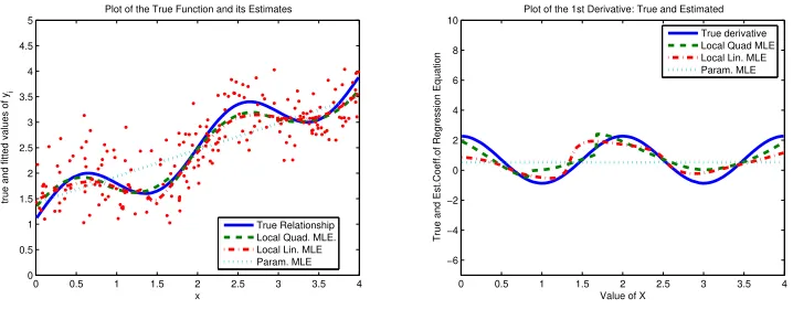
Example 4. Periodic Model with Heteroskedasticity

In this scenario we assume the regression function has some periodicity. In particular, we assume that

f(Xi) =β0+β1sin(γXi) +β2Xi, i= 1, . . . , n. (4.3)

Figure 5 shows a typical estimation result for n = 200. The specific values of the parameters in this example are β0 = 1.1, β1 = 0.5, β2 = 0.7, γ = π and Xi ∼ U(0,4).

Moreover, to complicate the estimation problem, we also assume heteroskedasticity ofσε. In

the illustration we choseσε = 0.25

√

6−Xi, so that the closer to the truncation bound, the

higher is the variance.

0 0.5 1 1.5 2 2.5 3 3.5 4 0

0.5 1 1.5 2 2.5 3 3.5 4 4.5 5

x

true and fitted values of y

i

Plot of the True Function and its Estimates

True Relationship Local Quad. MLE. Local Lin. MLE Param. MLE

0 0.5 1 1.5 2 2.5 3 3.5 4 −6

−4 −2 0 2 4 6 8 10

Plot of the 1st Derivative: True and Estimated

Value of X

True and Est.Coeff.of Regression Equation

True derivative Local Quad MLE Local Lin. MLE Param. MLE

Figure 5: Example 4: periodic model with heteroskedastic shape parameter. Left panel is the model and right panel is the derivative.

Again, we see some oversmoothing of the hurdles or bumps but we still capture the essence of the shape quite well. Again not surprisingly, the quadratic approximation exhibits better performance than the linear one for estimation of both the regression equation and its derivative. Also we note that that the fit of derivative appears not as good as the fit of the regression function itself, due to the differences in rates of convergence of these estimators. This should be expected as a rule, due to the fact that the higher the order of the derivative (0vs. 1 in our case), the lower the speed of convergence of the estimator, as clearly stated in our Theorem 3.1.

4.5

Example 5. Multivariate Model with Heteroskedasticity

Here we consider two regressors that influence the dependent variable through a quadratic form. We want to see how our estimators perform for this type of scenario because theU -shape relationships are fairly common in economic phenomena. In addition, we want to see the performance when the situation is complicated by dependence of the variance on some of the regressors. For example, the employment level in a company may positively influence not only the mean of inefficiency but also companys risk (variance) of being inefficient,

e.g., because of increased risk of principal-agent problems, of pressure from trade unions, of strikes, etc. . . Formally, our scenario is given by (4.1), where fori= 1, . . . , n:

f(Xi) =β0+β11X1i+β12X12i+β21X2i+β22X22i+γX1iX2i (4.4)

withσε(Xi) =σ−ζ(X1i+δ)2.

−0.1, β12= 0.2, β21 =−0.1, β22 = 0.2, γ =−0.1, σ = 0.3, ζ = 0.05, δ = 1 and n= 200. Note that for these particular values, heteroskedasticity is such that the variance increases near the truncation level, which complicates the estimation problem (homoskedastic case was also studied and good performance was also observed but to save space and we do not present them). We see that the performance of the local linear is fairly good, but the quadratic one is much better.

−2 −1 0 1 2 −2 −1 0 1 2 1 1.5 2 2.5 3 3.5

1.2 1.4 1.6 1.8 2 2.2 2.4 2.6 2.8 3 1.2 1.4 1.6 1.8 2 2.2 2.4 2.6 2.8 3

true values of y

fitted values of y True vs. Fitted via different methods

LLQuad. fit LLLinear fit

Figure 6: Example 5: Multivariate model with heteroskedastic shape parameter. Left panel is the model and right panel is the obtained fit.

Figure 7 gives a sense of the fit of the estimates of the partial derivatives of f w.r.t. X1

and X2 , respectively. We see that the quadratic approximation substantially outperforms the linear one.

−1 −0.5 0 0.5 1 −1 −0.8 −0.6 −0.4 −0.2 0 0.2 0.4 0.6 0.8 1

true values of derivative of y

fitted values of derivative of y True vs. Fitted via different methods

LLQuad. fit LLLinear fit

−1 −0.5 0 0.5 1 −1 −0.8 −0.6 −0.4 −0.2 0 0.2 0.4 0.6 0.8 1

true values of derivative of y

fitted values of derivative of y True vs. Fitted via different methods LLQuad. fit

LLLinear fit

Figure 7: Example 5: Multivariate model with heteroskedastic shape parameter. Fit of the partial derivatives of f w.r.t. X1 (left panel) andX2 (right panel).

reasons. First of all, the true model is quadratic and so it is natural that the local quadratic fit is better than the local linear one. Second, and more generally, the (finite-sample) bias of our estimator reduces with the order of local approximation of our estimator, as precisely stated in our Theorem 2.1. It is known that the higher the order approximations the better shall be the fit (e.g., see Fan and Gijbels, 1996). In practice, however, researchers often stay satisfied with local linear estimators, motivating it with similar asymptotic properties but relative computational simplicity.

All our simulations suggest a different practical conclusion: One should definitely prefer the local quadratic likelihood estimator of the regression function relative to the local linear one, despite the increased computational complexity. This is especially true for the following cases: (i) when heteroskedasticity is expected; (ii) when one has many regressors with pos-sible interaction among them; (iii) when the goal is to estimate the first partial derivatives of the regression function. And, these cases, are more the rules than exceptions in empirical studies. Higher order approximations (especially odd-order) theoretically should give better fit. However, even for third-order approximation, the programming cost and optimization cost increase dramatically and might not worth further improvements in the fit.

5

An Empirical Illustration

The goal of this section is not to make a solid empirical investigation but to get a feeling of the use and value of our estimator in studying economic phenomena. For this, we use data from a study about economic growth in the world, by Kumar and Russell (2002) that received considerable attention in the recent literature. Specifically, we take their estimated Farrell/Debreu-type efficiency scores for 57 countries in the world and relate it to capital-labor ratio (in the year 1990) in these countries1_.

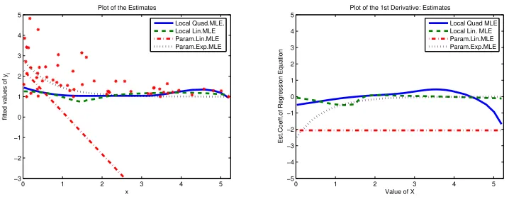
We first use the same three estimators as in the simulations and obtain quite interesting results, presenting them in Figure 8. First of all, recall that the main argument of Kumar and Russell (2002) was that the change in capital per labor was the major source of eco-nomic growth in 1965-1990 and especially of the change from uni-modality to bi-modality of distribution of income per worker. The fully parametric linear model tells us that there is also negative (positive) relationship between the inefficiency (efficiency) of a country and its capital intensity. That is, the more capital per labor in a country the less inefficiency (the more efficiency) score of this country relative to the other countries. The estimated2 _slope

1_{In the regression estimation we had to drop one observation (Switzerland) that appeared to be an outlier}

in terms of capital per worker and so causing computational problem in optimization of the likelihood function (even in fully parametric case).

parameter is 2.

0 1 2 3 4 5

−3 −2 −1 0 1 2 3 4 5

x

fitted values of y

i

Plot of the Estimates

Local Quad.MLE. Local Lin.MLE Param.Lin.MLE Param.Exp.MLE

0 1 2 3 4 5

−5 −4 −3 −2 −1 0 1 2 3 4 5

Plot of the 1st Derivative: Estimates

Value of X

Est.Coeff.of Regression Equation

Local Quad MLE Local Lin. MLE Param.Lin.MLE Param.Exp.MLE

Figure 8: Empirical illustration. Left panel is the model and right panel is the derivative.

On the other hand, observing the left panel of Figure 8, one can see that heteroskedas-ticity is likely to be present in data: the less capital-labor the larger is the variance of inefficiency variable. So the apparent negative relationship can in fact be a result of severe heteroskedasticity.

From the plot of the linear fit in Figure 8, we might guess that the linear parametric model might be inappropriate here, and exponential might be a better choice. Of course, in practice such visually based conclusions on the parametric form can hardly be done for multivariate regressions, but this is useful for illustration and discussion here. We thus estimated the exponential (homoskedastic) model, Y = 1 + exp(X _∗β) + ε, which corresponds to the dotted curves in Figure 8. We see that the relationship between the capital depth and the inefficiency is indeed suggested to be negative, with relatively high marginal effect at the low capital per worker ratio and monotonically decreasing to almost no effect at the higher levels. We could also try various forms of heteroskedasticity with this or another functional form, but guessing about the two functional forms for the regression and for the shape parameter at the same time might be too much for a scientific approach.

So, instead, we try our non-parametric procedure that is capable of handling heteroskedas-ticity of unknown form and we get quite different conclusion than what the parametric models told us. Both linear and quadratic local likelihood estimators suggest that there is virtually no relationship between the Farrell/Debreu-type efficiency score of a country vs. capital-labor of this country. Specifically, the fitted curve characterizing the relationship is almost flat and the slope coefficient is fluctuating near zero. We see an exception at the very end

(top 10% percentile) of the empirical range of the explanatory variable, where the quadratic approximation suggests that the relationship might indeed be negative, but this is only in a small interval where there is only a few observations.

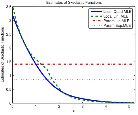
The results from estimating the regression equation non-parametrically makes us conjec-ture that the negative relationship between countries inefficiency score and its capital-labor ratio is coming not through the level (mean) of inefficiency but through the dispersion of inefficiency. Intuitively, we can say that the less capital-labor in a country the greater is the

riskof having high inefficiency score for that country. Figure 9 gives a plot of the estimated variance of the error termvs. the explanatory variable, which supports our conjecture.

0 1 2 3 4 5

0 0.5 1 1.5 2 2.5 3 3.5

x

Estimates of Skedastic Functions

Estimates of Skedastic Functions

Local Quad MLE Local Lin. MLE Param.Lin.MLE Param.Exp.MLE

Figure 9: Empirical illustration. Estimation of the heterskedastic shape function.

The result we obtained in our small application is consistent with capitalist philosophy: if people possess a lot of capital within a country then they have a lot of incentives to create a political system that would minimize the risk of underutilization (inefficiency) of their capital. On the other hand, if people possess little of capital, “they have got little to lose!”, and so not as much interested in building appropriate institutions that would protect property rights and so minimize the risk of underdevelopment. Looking at the data confirms that it is mostly the underdeveloped countries that are in the range of high variance of inefficiency scores and low capital per labor levels.

our estimator in practice and show how it could suggest radically different conclusions than those obtained from commonly used parametric methods.

6

Concluding Remarks

In this work we proposed a fairly flexible estimator for the context of truncated regression that does not require parametric assumptions. For this, we extended the theory of local

maximum likelihood estimation, in particular the recent work of Kumbhakar et al. (2006), to the truncated case. We provided the asymptotic results of our estimator. Specifically, the estimator is consistent and asymptotically normally distributed with variance that can be estimated from data.

We also illustrated the performances of two variants of our estimator (namely, linear and quadratic approximations) on various simulated data sets, comparing it to the truth and to the parametric estimator. Remarkably, for the univariate case, our estimator performs as good as the traditional, fully parametric estimator when the assumptions for the latter hold,

i.e., we do not lose virtually anything by allowing the flexibility. However, our estimator performs much better when the parametric assumptions on the regression equation does not hold or even only when the assumption of homoskedastic shape parameter of the error term does not hold. We also illustrated the use of our estimator on a real data set from the recent study of Kumar and Russell (2002), analyzing relationship between the efficiency scores and the capital deepness in countries in the world. In this application we noticed that quite different and perhaps more plausible implications can be inferred using our estimator instead of the commonly used parametric one.

It became common that empirical researchers often are satisfied with local linear estima-tors, motivating it with similar asymptotic properties but relative computational simplicity. However, all our simulations suggested that, despite some increase in the computational complexity, the local quadratic likelihood estimator of the regression function should be pre-ferred relative to the local linear one, especially if heteroskedasticity is expected and certainly when the focus is on estimating first derivatives.

study is just the start, telling that the non-parametric estimator in the truncated regression context should exhibit a fair degree of robustness to various deviations from linearity in the regression equation and in the function defining the heteroskedastic shape parameter and thus shall prove to be very useful in practical applications.

7

Regularity Conditions and Proof of Theorems

7.1

Regularity Conditions

First, we collect the assumptions for Theorem 3.1. Fora_∈IRr(p) and b _∈IR, let ψ(a, b_|x)_≡ [ψ1(a, b_|x), ψ2(a, b_|x)]T where

ψ1(a, b|x) = Ehℓ10 Y, f(x) +a0+a1u1+· · ·+ar(p)−1upd, τ +b

X =x

i

,

ψ2(a, b_|x) = Ehℓ01 Y, f(x) +a0+a1u1+_{· · ·}+ar(p)−1up_d, τ +b

X =x

i

.

(A1) Q(a, b) = 0 has the unique solution a= 0 _∈IRr(p) and b = 0_∈IR;

(A2) sup_(aT_,b)T_∈A

ψ(a, b|x+z)−ψ(a, b|x)

→ 0 as z → 0 for some compact set A ⊂

IRr(p)+1;

(A3) for (i, j) = (1,0) and (0,1), the following condition holds: for any compact sets

A1,A2 ⊂IR, there exist functions Uij such that supν∈A1,ω∈A2|ℓij(y, ν, ω)| ≤Uij(y) and sup_|z−x|≤εE U2+δ

ij (Y)|X =z

<_∞ for some ε, δ >0;

(A4) for (i, j) = (2,0), (0,2) and (1,1), the following condition holds: ℓij(y, ν, ω) are

continuous in (ν, ω) for eachy, and for any compact sets_A1,_A2 ⊂IR, there exist

func-tionsUij such that supν∈A1,ω∈A2|ℓij(y, ν, ω)| ≤ Uij(y) and sup|z−x|≤εE U

2

ij(Y)|X =z

<

∞ for some ε >0;

(A5) g(x) > 0, ρ20(x) > 0, ρ20(x)ρ02(x)−ρ11(x)2 _{> 0, v20(x) > 0, v20(x)v02(x)−} v11(x)2 _>0

(A6) g, all ρij and vij for (i, j) = (2,0),(0,2),(1,1) are continuous at x;

(A7) K is nonnegative, bounded and supported on [₋1,1]d_;

(A8) The function f has (p+ 1)th continuous partial derivatives at x;

Now, to list the assumptions for Theorem 3.2, let ψ(a, b|x)≡[ψ1(a, b|x), ψ2(a, b|x)]T for

a_∈IRr(p) and b_∈IRr(q), where

ψ1(a, b_|x) = Ehℓ10 Y, f(x) +a0+a1u1+_{· · ·}+ar(p)−1upd,

τ(x) +b0+b1u1+· · ·+br(q)−1uqd

X =x i

,

ψ2(a, b|x) = Ehℓ01 Y, f(x) +a0+a1u1+· · ·+ar(p)−1upd,

τ(x) +b0+b1u1+_{· · ·}+br(q)−1uq_d

X =x

i

.

(B1) Q(a, b) = 0 has the unique solution a= 0_∈IRr(p) and b = 0_∈IRr(q);

(B2) sup_(aT_,bT₎T_∈A

ψ(a, b|x+ z) −ψ(a, b|x)

→ 0 as z → 0 for some compact set

A ⊂ IRr(p)+r(q);

(B3)–(B7) same as (A3)–(A7);

(B8) The function f has (p+ 1)th continuous partial derivatives, and the function τ

has (q+ 1)th continuous partial derivatives, at x;

(B9) h→0 and nh→ ∞ as n→ ∞, and nh2(p∧q)+d+2 _{< C for some positive constant} C.

7.2

Proof of Theorem 3.2

We outline a proof of Theorem 3.2 only. Proof of Theorem 3.1 is similar and less involved than that of Theorem 3.2.

Define u(j) _{= u}ξj(1), . . . , uξj(mj)T for a d-vector u, where ξ

j(s) is defined in Section 3.

Let ˜f be the pth order polynomial approximation of f around the point x, and ˜τ the qth order polynomial approximation ofτ, i.e.,

˜

f(u) =

p X

j=0

θ(j)(x)T(u₋x)(j),

˜

τ(u) =

q X

j=0

τ(j)(x)T(u−x)(j),

whereθ(j)_{(x) is defined at (3.1). Define}

ˆ

a(j) _≡ˆa(j)(x) =hjθˆ(j)(x)₋θ(j), j = 0, . . . , p,

ˆ

b(j)_≡ˆb(j)(x) =hj τˆ(j)(x)₋τ(j)

Also, define

Zp,i =

1,

Xi1−x1 h

, . . . ,

Xid−xd

h

pT

,

˜

ℓjk(i, a, b) = ℓjk

Yi,f˜(Xi) +a0 +a1

Xi1−x1 h

+_{· · ·}+ar(p)−1

Xid−xd

h

p

,

˜

τ(Xi) +b0+b1

Xi1−x1 h

+· · ·+br(q)−1

Xid−xd

h

q

Q1n(a, b) = n−1 n X

i=1

Zp,iℓ10˜ (i, a, b)Kh(Xi−x),

Q2n(a, b) = n−1 n X

i=1

Zq,iℓ01˜ (i, a, b)Kh(Xi−x).

Write ˆa = (ˆa(0)T_{, . . . ,aˆ}(p)T₎T _{and ˆb = (ˆb}(0)T_{, . . . ,}ˆ_b(q)T₎T_{. Then (ˆa,}ˆ_{b) is the solution of the}

equation Qn(a, b) = 0, where Qn(a, b) = Q1n(a, b)T, Q2n(a, b)T T

is a [r(p) +r(q)]-vector. One can prove in a similar way as in Kumbhakaret al. (2006) that for any compact setA

sup

(a,b)∈A

Qn(a, b)−EQn(a, b)

= Op n

−1/2_h−d/2_(logn)1/2

, (7.1)

sup

(a,b)∈A

EQn(a, b)−Q(a, b)

= o(1). (7.2)

By (7.1), (7.2) and the assumption (B1) it follows that

ˆ

a=op(1), ˆb=op(1). (7.3)

Next, let Sn(a, b) be a [r(p) +r(q)]×[r(p) +r(q)] matrix defined as

Sn(a, b) = 



n−1Pn

i=1Zp,iZp,iT ℓ20˜ (i, a, b), n−1 Pn

i=1Zp,iZq,iT ℓ11˜ (i, a, b)

n−1Pn

i=1Zq,iZp,iT ℓ11˜ (i, a, b), n−1 Pn

i=1Zq,iZq,iT ℓ02˜ (i, a, b) 



It can be proved that for any compact set_A

sup

(a,b)∈A

Sn(a, b)−ESn(a, b)

=Op n

−1/2_h−d/2_(logn)1/2

(7.4)

A Taylor expansion ofQn(a, b) gives

0 =Qn(ˆa,ˆb) =Qn(0,0) +Sn(a∗, b∗) ˆ a ˆ_b , (7.5)

wherea∗ _andb∗ _{are random vectors such that|(a}∗T_{, b}∗T₎T_{| ≤ |(ˆa}T_,ˆ_bT₎T_{|. The consistency of}

(ˆa,ˆb) as given at (7.3) and the result (7.4) imply

Furthermore, one can show that

ESn(0,0) =−D(x)g(x) +o(1). (7.7)

By (7.5)–(7.7) and the fact thatQn(0,0) = Op(n−1/2h−d/2), we obtain the following expansion

for (ˆaT_,ˆ_bT₎T_:

ˆ

a

ˆ

b

=g(x)−1D(x)−1Qn(0,0) +op(n−1/2h−d/2). (7.8)

The mean and variance of (ˆaT_,ˆ_bT₎T _{come from those of Q}

n(0,0). One can show

E[Qn(0,0)] = "

hp+1_ρ20(x)N(p)

p+1θ(p+1)(x) +hq+1ρ11(x)N (p)

q+1τ(q+1)(x) hp+1_ρ11(x)N(q)

p+1θ(p+1)(x) +hq+1ρ02(x)N (q)

q+1τ(q+1)(x)

#

g(x) (7.9)

+o(hp+1+hq+1),

var[Qn(0,0)] = n−1h−d

M(p,p)_v

20(x) M(p,q)v11(x) M(q,p)_v

11(x) M(q,q)v02(x)

g(x) +o(n−1_h−d_{). (7.10)}

The asymptotic normality of Qn(0,0) follows from the assumption (B3) by a direct

ap-plication of the Lindeberg-Feller theorem. The theorem now follows from the asymptotic normality ofQn(0,0) and (7.8)–(7.10).

References

[1] Chambers, R.G., Y. Chung, R. F¨are (1996), Benefit and distance function, Journal of Econonomic Theory, 70, 407–419.

[2] Debreu, G. (1951), The coefficient of resource utilization,Econometrica, 19, 273–292.

[3] Carroll, R. J., Fan, J., Gijbels, I. and Wand, M. P. (1997), Generalized partially linear single-index models, Journal of the American Statistical Association, 92, 477–489

[4] Fan, J. and Gijbels, I. (1996),Local Polynomial Modelling and Its Applications, Chapman and Hall, London.

[5] Fan, J., Heckman, N. E and Wand, M. P. (1995), Local polynomial kernel regression for generalized linear models and quasi-likelihood functions, Journal of the American Statistical Association, 90, 141–150.

[7] Kumar, S. and R.R. Russell (2002), Technological Change, Technological Catch-up, and Capital Deepening: Relative Contributions to Growth and Convergence, American Eco-nomic Review, 92, 3, 527–548.

[8] Kumbhakar, S. C., Park, B. U., Simar, L. and Tsionas, E. G. (2006), Nonparametric stochastic frontiers: a local maximum likelihood approach, Journal of Econometrics, forthcoming.

[9] Lewbel, A. and O. Linton, (2002), Nonparametric censored and truncated regression,

Econometrica, 70, 765–779.

[10] Luenberger, D.G. (1994), Optimality and the theory of value,Journal of Econonomic Theory, 63, 147–169.

[11] Simar L. and P. Wilson (2006), Estimation and inference in two-stage, semi-parametric models of production processes, Discussion Paper (0307) of Institute of Statistics, Uni-versity Catholique de Louvain, Journal of Econometrics, forthcoming.

[12] Tibshirani, R. and Hastie, T. J. (1987), Local likelihood estimation, Journal of the American Statistical Association, 82, 559–567.