Measuring Dependence Risk of Funds with Copula in China

(1)

http://dx.doi.org/10.4236/am.2014.513179

Measuring Dependence Risk of Funds with

Copula in China

Jiaqi Tang1_{, Guohua Sun}2

1_{School of Management, Guilin University of Technology, Guilin, China} 2_{College of Science, Guilin University of Technology, Guilin, China}

Email: 262605708@qq.com, 296231428@qq.com

Received 24 April 2014; revised 3 June 2014; accepted 15 June 2014

This work is licensed under the Creative Commons Attribution International License (CC BY).

http://creativecommons.org/licenses/by/4.0/

Abstract

The aim of this paper is to measure dependence risk of fund market with copulas in China. Firstly, we introduce several common copula functions, then estimate parameters of copula function, and discuss how to select the optimal copula function. Finally, according to Shanghai and Shenzhen fund data, empirical analysis was done. Different combinations of risk values were obtained.

Keywords

Copula, Dependence Risk, Monte Carlo Simulation, Parameter Estimation

1. Introduction

(2)

we analyzed copula functions and their characteristics of the application on correlation analysis, then selected the appropriate copula function and got different combinations of risk values.

2. Introduction to the Theory of Copulas

2.1. The Definition and Properties of Copulas

In 1959, Abe Sklar first proposed copula function, but financial experts didn’t pay attention to copula function until the 1990s. As a method to research associated structures of random variables, copula has its unique properties, namely multivariate distribution function can be described by univariate marginal functions and multivariate correlation structure functions.

Sklar Theorem [1]: Set F x x

(

1, 2,⋅⋅⋅,xn

)

as N-dimensional distribution function whose marginal distribution

is F x1

( ) ( )

1 ,F2 x2 ,,Fn

( )

xn , then there exists a function C

( )

⋅ which has only copula expression:

(

1, 2, , n

)

(

1

( ) ( )

1 , 2 2 , , n

( )

n

)

F x x ⋅⋅⋅ x =C F x F x ⋅⋅⋅ F x (1)

According to Sklar theorem, we can through copula function C

( )

⋅ and marginal distributions to build multi-variate joint distribution. Since the marginal distribution function arbitrary value F xi

( )

i

(

i=1, 2,⋅⋅⋅,n

)

can be regarded as uniformly distributed random variable values of Ui on I =

[ ]

0,1 , denoted

1

F− _{is inverse function} of F, namely _F−1

( )

_u ₌_inf

{

_{x F x}

( )

_≥_u

}

, assuming marginal distributions F x1

( ) ( )

1 ,F2 x2 ,,Fn

( )

xn are con-tinuous, then by the Sklar’s theorem, there exists a unique copula function C

( )

⋅ , making

(

)

(

)

(

1

( )

1

( )

1

( )

)

1, 2, , 2 1, 2, , n 1 1 , 2 2 , , n n

C u u ⋅⋅⋅u =F x x ⋅⋅⋅x =F F− u F− u ⋅⋅⋅F− u (2)

Use type (2), we could start with the marginal distribution and the dependency structure processing, respec-tively, to integrate, can more effectively and to explore the common changes of relationship between variables, and then get more suitable joint probability distribution and risk assessment as a portfolio or commodity pricing.

2.2. Several Kinds of Commonly Used Copulas Function

There are many kinds of copulas function, basically we are commonly used is Elliptic Copulas and Archimedean Copulas. And in each group, there are a number of specific copulas connect functions. Different copulas connect functions have different nature. In practical application, how to choose the right copulas connect function needs to follow the two principles below: one is copulas connect model should be easy to operate and understand, avoid the phenomenon of unknown parameters of significance [5]; the other one is to select the copula function which can adapt to related structures of the sample data. The Elliptic Copulas has the property of symmetric tail dependence, it violates the fat-tailed distribution of financial data. Currently, the most widely applied in the field of financial category is the Archimedean Copula function. What’s more, its structure and computation are simple. Therefore, here are several kinds of commonly used Archimedean copulas connect function, this paper just considers the binary case.

1) Gumbel Copula Function

The distribution function is expressed as follows:

( )

(

) (

)

1

, exp ln ln , 1

Gu

C_θ u v = _− − u θ+ − vθ θ_ θ≥

  (3)

The Gumbel Copula function is very sensitive to the changes of the variables at the up-tail of the distribution, so it can fast capture the variations which dependent on the up-tail. It can be used to describe the dependencies be-tween financial variables with relevant characteristics of the up-tail. The Parameter θ describes the extent of their dependency, when θ =1, the variable will be independent. When θ→ ∞, the Variable tends to com-pletely dependent.

2) Clayton Copula Function

( )

(

)

1

, 1 , 0

Cl

C_θ u v = u−θ+v−θ− −θ θ> (4)

(3)

so it can fast capture the variations which dependent on the down-tail. It can be used to describe the dependencies between financial variables with relevant characteristics of the down-tail. When θ =0, it represents independent variables ;When θ → ∞, it represents that the variables are completely dependent.

3) A12 Copula Function

( )

_, ₁

(

1 ₁

) (

1 ₁

)

1 1_, ₁

C u v u v

θ θ θ θ θ − − −  _ _  = +_ _ − + − _ _ ≥  

  (5)

The Gumbel Copula function only with the up-tail dependence, on the contrary, the Clayton Copula function only with the down-tail dependence. But the A12 Copula function owns these two characters at the same time.

4) Frank Copula Function

( )

1

(

e 1 e

)(

1

)

{ }

, ln 1 , R\ 0

e 1

u v

C u v

θ θ θ θ θ − − −  ₋ ₋    = − + ∈  −    (6)

The density function’s distribution of Frank Copula function was “U” shaped and its distribution has symmetry. So we cannot capture the asymmetric dependencies between random variables [6].

The above selected some kinds of Copula function with different characteristics in Archimedean Copula func-tion family. In fact, it can make great influence on the structure of joint distribufunc-tion when we select different Copulas functions and marginal distribution.

2.3. The Parameter Estimation Method and Selection Principle of Copula Function

For parameter estimation of the specific copula function, we can use the parametric approach and the nonpara-metric approach averagely: 1) The EML method and the IFM method are more commonly used in the paranonpara-metric approach. The EML method can estimate the marginal distribution and the parameters in copula function simul-taneously. The estimation process is divided into two steps by the IFM method. Firstly, to estimate the parameters of marginal distribution function. Then we need to estimate the parameters of copula function. 2) The Genest and Rivest method are more commonly used in the nonparametric approach [7]. If there are too many parameters in the marginal distributions and copula functions, it is very hard to calculate the exact value of EML. Because of this fact, we use the IFM to estimate the parameter θ of copula function in this paper. The estimation principle of IFM is to make the parameters of marginal distribution function and copula function estimated in two steps, it is usually also called two-stage estimation method.

First of all, we need to estimate the marginal distribution functions FX and FY, FX and FY can use the parameter model, such as the Normal distribution, the Students-t distribution, the generalized Pareto distribution and so on. Set the estimation is FˆX , FˆY. Then, for this FˆX , FˆY, to construct pseudo samples from the copula below [8]:

(

_{ˆ ˆ}_,

)

(

ˆ

( )

_,ˆ

( )

)

_{1, 2,} _,

i i X i Y i

u v = F x F y i= ⋅⋅⋅n (7)

Secondly, for the copula C u v

(

, ;θ

)

which has the distribution density function c u v

(

, ;θ

)

and unknown parameter θ, we need to construct the logarithm likelihood function

(

)

(

)

1

ˆ ˆ, ; ln ˆ ˆ, ; 1, 2, , n

i i i

l u vθ c u v θ i n

=

∑

= ⋅⋅⋅ (8)

In the end, through standard numerical calculation to find the maximum value, we can get the estimate value of the parameter θ.

3. The Selection of Copula Function

3.1. The Statistical Description and Analysis of Fund Yield

(4)

by its logarithmic transformation, we can get a corresponding logarithmic revenue rate is

(

x yi, i

)

=

(

log

(

pi+1 pi

)

, log

(

qi+1 qi

)

[9]. First of all, the basic statistics of the Shanghai fund yield and Shenzhen fund yield were calculated, the results are shown inTable 1.

FromTable 1, we can see that normality assumption is not appropriate for two kinds of index of yield. Come back now we discuss the two funds dependent risk measurement problem, to analyze their gap between joint distribution and normal distribution. Firstly, we calculate the degree of dependency of these two funds quantita-tively. Set X represents the Shanghai stock market fund yields and Y represents the Shenzhen stock market fund yields, it is easy to calculate the correlation coefficient ρ

(

X Y,

)

=0.9591, rank correlation coefficient

(

,

)

0.9496 s X Y

ρ = , Kendall τ=0.8172. This illustrates that there is a strong linear correlation in the yield of these two kinds of funds. What’s more, ρs and

τ

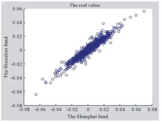
are smaller than classical linear correlation coefficient. In order to further illustrate the gap between the joint distribution and the normal distribution of these two kinds of yield, we made the scatterplot of these two kinds of yield. In addition, we also made the simulation diagram of the bivariate normal distribution which structured by the mean and covariance of these two yields, as shown inFigure 1 andFigure 2.

FromFigure 1 andFigure 2, it’s easy to see that the difference is quite obvious in the tail of the two distribution of data. It shows that using bivariate normal distribution to describe the distribution of these two funds yield is obviously inaccurate. It also suggests that using classical linear correlation coefficient to measure dependency is not enough. So, we use the copula function to measure the dependent risks of this two yields.

3.2. The Selection of Copula Function

Now let’s consider the problem how to select copulas function C

( )

⋅ . Based on the marginal distribution extra-polation, first of all, to structure the sample points which based on the following change:

(

_{ˆ ˆ}_,

)

(

ˆ

( )

_, ˆ

( )

)

_{1, 2,} _,

i i X i Y i

u v = F x F y i= ⋅⋅⋅n

[image:4.595.89.540.432.706.2]

When considering the risk management is only interested in the distribution of the tail, but a large number of studies have shown that yields on the tail of the distribution is the generalized Pareto distribution (GPD), so

Table 1. Basic statistical description of the fund yield.

Fund Type N Mean (%) Standard

Deviation (%) Partial Degrees Kurtosis JB Statistic

Shanghai Fund 997 0.0423 1.3819 −0.0071 2.6022 7.9231

Shenzhen Fund 997 0.0562 1.2527 −0.0934 2.4705 15.7597

(5)

[image:5.595.184.446.83.280.2]

Figure 2. The simulation diagram of the bivariate normal distribution of Shanghai fund and Shenzhen fund.

( )

ˆ X i

F x , FˆY

( )

yi will be taken for the GPD distribution function of the two yields, then according to the mar-ginal distribution extrapolation method to estimate the parameters in the function [8]. Meanwhile, as we care about its risk, so take x, y for the opposite number of its yield. We select Gumbel, Clayton, A12 and Frank Copula to estimate and fitting respectively, after that, according to the AIC and BIC rules to select the most appropriate copulas and its parameters [10]. The specific results are shown inTable 2.

FromTable 2, it can be seen that the AIC and BIC of Clayton Copulas function are minimal. In view of this, we choose Clayton Copulas function to measure the dependent risks of Shanghai, Shenzhen fund yields.

4. The Dependent Risk Measure in Two Kinds of Fund Portfolio

Assuming in a period of time, to invest in assets 1 and 2, set α1 and α2 represent the proportion of two kinds of

asset investment respectively, X and Y represent the logarithmic yield of this two kinds of asset respectively. Then, the logarithmic yield of this two kinds of asset portfolio can be expressed as below:

(

1 2

)

ln eX eY

R= α +α

Due to the nonlinear transformation of combination between X and Y is R, and it is impossible to know the distribution of R. So, it is hard to calculate the dependent risk directly. But, we can use copulas connection func-tion to measure the risk. Here we use copula method to do the Monte Carlo simulafunc-tion. The algorithm of simula-tion method is as follows [4]:

1) Generate two uniform random numbers u, w_;

2) Make the first random number for asking is x F1 1

( )

u

−

= ;

3) Through the selected copulas connect function to obtain the random number on uniform distribution which is located in the second sequence v Cu1

( )

w

−

= (Among C_u= ∂C u v

( )

, ∂u); 4) By calculating to obtain the second random number, it is y F2 1

( )

v

−

= .

For the Combination yields R, the VaR and ES which gave them the confidence probability q are

( )

1

VaRq FR q

− −

= (9)

(

)

(6)

Table 2. The parameter estimation under the different copulas function.

Copula AIC BIC θ

Gumbel −634.7526 −629.2547 5.4705

Clayton −767.4137 −762.6352 8.9409

A12 −579.6481 −574.8916 3.6470

[image:6.595.89.538.100.318.2]

Frank −548.8514 −543.3805 8.4531

Table 3. The VaR of fund yield.

Combination ratio VaR0.95 VaR0.99 VaR0.999 ES0.95 ES0.99 ES0.999

1 0.9 2 0.1

α= α = 0.1237 0.1867 0.3308 0.1613 0.2255 0.7537

1 0.7 2 0.3

α = α = 0.1137 0.1640 0.2737 0.1436 0.1954 0.6241

1 0.5 2 0.5

α = α = 0.1061 0.1509 0.2131 0.1349 0.1762 0.5616

1 0.3 2 0.7

α = α = 0.0996 0.1530 0.2263 0.1307 0.1799 0.5847

1 0.1 2 0.9

α= α = 0.0912 0.1604 0.2756 0.1320 0.2004 0.6358

5. Conclusion

In recent years, the copulas function technology applied in the financial aspects has achieved great development, But the study of copulas connect function is still in its infancy in China at present. This article first introduced several kinds of commonly used copulas connect function, then used the marginal distribution extrapolation for parameter estimation, and selected the optimal copula function. Finally, the VaR and ES values of different combinations between Shanghai fund logarithm yield and Shenzhen fund logarithm yield were calculated by using the copula function theory and combining with Monte Carlo simulation method. By this way, we can measure the dependent risk of fund market well. With the research on copula function being increasingly mature, the copula function will become a powerful tool in the field of finance to greatly promote the stable development of the financial sector.

Fund Project

The national natural science fund project (11061012); The projects of spatial information and surveying- map-ping key laboratory in guangxi (GKN 1103108-20); The research projects of Guilin technology bureau (20110120-5).

References

[1] Sklar, A. (1959) Functions de Repartition an Dimension Set Leursmarges. Publications de L’In-stitut de Statistique de L’Universite de Paris.

[2] Nelsen, R.B. (2006) An Introduction to Copulas. Springer-Verlag, New York.

[3] Bouye, E., Durrleman, V., Nikeghbali, A., et al. (2000) Copulas for Finance: A Reading Guide and Some Application. Working Paper, City University Business School-Financial Econometrics Research Centre, Londres.

[4] Chen, S.D., Hu, Z.Y. and Kong, F.L. (2006) Using Copula Function to Measure the Monte Carlo of Risk Value. Social Science Journal of Jilin University, 46, 85-91.

[5] Rosenberg, J.V. and Schuermann, T. (2006) A General Approach to Integrated Risk Management with Skewed, Fat- tailed Risks. Journal of Financial Economics, 79, 569-614.http://dx.doi.org/10.1016/j.jfineco.2005.03.001

[6] Li, S. and Lu, Z.D. (2008) The Copulas Connect Function in the Application of the Measure on Risk Value. The Fi-nancial Management, 20, 10-16.

[7] Genest, C. and Rivest, L.P. (1993) Statistical Inference Procedures for Bivariate Archimedean Copula. Journal of the American Statistical Association, 8, 1034-1043.http://dx.doi.org/10.1080/01621459.1993.10476372

(7)

Co-pulas Connect Method. Statistical Research, 25, 82-85.

[9] Li, Y. and Cheng, X.J. (2006) The Copulas Connect Tail Correlation Analysis of the Shanghai Composite Index and Hang Seng Index. Systems Engineering, 24, 88-92.

(8)

currently publishing more than 200 open access, online, peer-reviewed journals covering a wide range of academic disciplines. SCIRP serves the worldwide academic communities and contributes to the progress and application of science with its publication.

Other selected journals from SCIRP are listed as below. Submit your manuscript to us via either