Bulk Arrival with working vacation

Bulk Arrival with working vacation

Dr. Naveen Kumar

Department of Applied Sciences, Bahra Institute of Management and Technology, Chidana

Email: naveenkapilrtk@gmail.com

Abstract

—

Here arrivals of the customer follow poisson distribution and there is single server who is

providing service to the customer. Also server serve the customer on first come first serve basis. The vacation queues

have been extended to computer networks, communications systems, as well as production management, inventory

management and other fields (Doshi B.T., 1990). For the classical single-server vacation model, a server stops

working completely during the vacation periods. However, the server can be generalized to work at a different rate

during the vacation periods. This type of queueing models are useful to analyze a variety of multi-queue systems that

frequently arise in computer and communication networks. Different parameter is used for finding expected busy

period and queueing length.

Keywords

—

Arrival pattern is poisson, Removable server, Service time is exponential distribution, queue discipline is FCFS, Stochastic process.

I.

INTRODUCTION

In this paper, the arrivals process is assumed to be Poisson with parameter  and the service by a single server. If the queue is empty then server goes on vacation, when the queue size is less then ‘a’ the server is on working vacation & if the queue size is > ‘a’ then server is busy. The server serve the customer according to exponential law with parameter 1 if server is on working vacation & the server serve the customer according to exponential law with parameter 2 if server is busy. For example, the allocation of the real time of a processor within a large switch or the allocation of the bandwidth of the bus of a LAN. In such systems, each queue may be processed either at a fast service rate or a nominal service rate depending on whether it acquires a token or not: That is, a queue operates at its fast service rate as soon as it gets the token. The scheduling discipline is exhaustive. In an exhaustive schedule, a queue possesses the token until the queue is empty. And then, the token is passed to the next queue. From the point of view of the individual queue, the server follows a working vacation. The server works at a slower rate rather than completely stops during a vacation. Such type of situation are called working vacation. Liu, Xu and Tian (2002), Takagi (2006), W.D. (2006), Servi, L.D. (2002) are discussed some working vacation queue.

Assumptions: The following assumption describe the system

1) Arrivals arrive according to poisson law with parameter  2) The service time distribution is exponentially with rate 1 and 2 3) Server serve the customer of batch sized if server is busy 4) Server serve the customer single if batch size is less than ‘a’ 5) The Queue discipline is first come first serve

6) The various stochastic process in the system are statistically independent 7) The server is removed from its service as soon as the Queue is empty.

II.

Analysis of Model

Pi,n(t) = P{x(t) = i, y(t) = n} x(t) = 0 y(t) = 0 vacation

The difference-differential equation governing the model are

)

t

(

P

00



= P00(t) + 1 P0,1(t) + 2 P0,2(t) …(1)

)

t

(

P

μ

)

t

(

P

μ

)

t

(

P

λ

)

t

(

P

)

μ

λ

(

)

t

(

P

₀



_,1







_0,1



₀₀



_{1 11}



_{2 12} …(2)

)

t

(

P

)

μ

λ

(

))

t

(

P

_n



_,1







_{1 n,1} +  Pn1(t) + 1Pn+1,11(t) 1  n  a  …(3)

)

t

(

P

₀



_,2 = ( + 2) P0,2(t) +  Pa1,1(t) + 2 Pn,2(t) n > a …(4)

2 , n

P



= ( + 2) Pn,2(t) +  Pn1,2(t) + 2 Pn+a,2(t) n  1 …(5) Taking Laplace Transformation of equation (1) to (5)

)

s

(

P

λ

)

0

(

P

)

s

(

P

S

₀₀



₀₀





_0,0 + 1

P

0,1

(

s

)



μ

2

P

0,2

(

s

)

(S + )

P

₀₀

(

s

)



1



μ

₁

P

₀₁

(

s

)



μ

₂

P

_0,2

(

s

)

P00(0) = 1 …(6)

)

1

)

s

(

P

μ

)

s

(

P

μ

(

λ

S

1

)

s

(

P

_{00 1 01}



_{2 02}







S

P

₀₁

(

s

)

 P01(0) = (+)

P

01

(

s

)



λ

P

00

(

s

)



μ

1

P

11

(

s

)



μ

2

P

12

(

s

)

 (S +  + )

P

₀₁

(

s

)



λ

P

₀₀

(

s

)



μ

₁

P

₁₁

(

s

)



μ

₂

P

₁₂

(

s

)

…(7)

)

s

(

P

μ

)

s

(

P

μ

)

s

(

P

λ

(

μ

λ

S

1

)

s

(

P

_{01 00}



_{1 11}



_{2 12}







)

s

(

P

μ

)

s

(

P

λ

)

s

(

P

)

μ

λ

(

)

0

(

P

)

s

(

P

S

_n,1



_n,1







_{1 n,1}



_n1,1



_{1 n1,1} + 2

P

n1,2

(

s

)

(S +  +1)

P

n1

(

s

)



λ

P

n1,1

(

s

)



μ

1

P

n1,1

(

s

)



μ

2

P

n1,2

(

s

)

…(8)

)

s

(

P

μ

)

s

(

P

μ

)

s

(

P

λ

(

μ

λ

S

1

)

s

(

P

_{n,1 n1,1}



_{1 n1,1}



_{2 n1,2}







)

S

P

_0,2

(

s

)



P

_0,2

(

0

)





(

λ



μ

₂

)

P

_0,2

(

s

)



λ

P

_a1,1

(

s

)



μ

₂

P

_n,2

(

s

))



(

S



λ



μ

₂

)

P

_0,2

(

s

)



λ

P

_a1,1

(

s

)



μ

₂

P

_n,2

(

s

)

))

s

(

P

μ

)

s

(

P

λ

(

)

μ

λ

S

(

1

)

s

(

P

_{a 1,1 2 n,2}

2 2

,

0



_

_





S

P

_n,2

(

s

)



P

_n2

(

0

)





(

λ



μ

₂

)

P

_n,2

(

s

)



λ

P

_n1,2

(

s

)



μ

₂

P

_na,2

(

s

)

…(9)

)]

s

(

P

μ

)

s

(

P

λ

[

)

μ

λ

S

(

1

)

s

(

P

_{n 1,2 2 n a,2}

2 2

,

n



_

_





 …(10)

 (S + +2)

P

n,2

(

s

)



λ

P

n1,2

(

s

)



μ

2

P

na,2

(

s

)

The characteristic equation from equation (10)

h(z) = 0

 2 z 2_

(S +  + 1)z +  = 0 …(11)

From (10)

(S + + 2)

P

n,2

(

s

)



λ

P

n1,2

(

s

)



μ

2

P

na,2

(

s

)

h(z) =  za+1 (S + + 2)z + 

h(z) = 0

 za+1 (S + +2) z +  = 0 …(12)

Suppose that f(z) = (S +  + 2) z and g(z) = za+1 + 

Consider the circle |z| = 1 where  is arbitrarily small & z = (1)ei, it can be shown that on the contour of the circle |g(z)| < |f(z)|

Hence by Rouche’s Theorem

f(z) and f(z) + g(z) will have the same number of zeros inside (z) = 1.

Since f(z) has only one zero inside the circle f(z) + g(z) = h(z) will also have only one zero inside (z) = 1, this root of h(z) = 0 is real and unique

iff  =

1

μ

a

λ

1



& (0 <  < 1)

and other roots i 1 Then  satisfies the equation

a =

α

1

)

α

1

(

α

μ

λ

a

1







=  + q +…+ a

and

α

1

)

α

1

(

α

μ

λ

a

2







From equation (11)

z =

2

2 2 1

μ

2

λ

μ

4

)

μ

λ

S

(

)

μ

λ

S

(













Let

 =

2

2 2 1

μ

2

μ

4

)

μ

λ

S

(

)

μ

λ

S

(













 =

2

2 2 1

μ

2

μ

4

)

μ

λ

S

(

)

μ

λ

S

(













Let  is the unique positive real root Hence by Rouche’s theorem

n 2 2 , 0 1

, 0 1

,

n

(

s

)

P

(

s

)

α

P

(

s

)

μ

R

P





1 a

1 2

2 , 0 1 1

, 0 1

, 1

i

R

μ

λ

S

λ

μ

)

s

(

P

μ

λ

S

λ

α

)

s

(

P

)

s

(

P

_ 



































































































n 2 1 2 2 1 01 2 , 0

R

α

μ

λ

S

λ

μ

λ

S

λ

μ

1

α

μ

λ

S

λ

μ

λ

S

λ

α

)

s

(

P

)

s

(

P

Let D1 =

]

R

α

λ

μ

)

μ

λ

S

)(

μ

λ

S

)[(

μ

λ

S

)(

μ

λ

S

(

)

μ

λ

S

)(

μ

λ

S

(

α

λ

n 2 2 2 1 2 1 2 1 2



























D1 = _{2 n}

2 2 1 2

R

α

λ

μ

)

μ

λ

S

)(

μ

λ

S

(

α

λ











From equation (6)

λ

S

1

D

).

s

(

P

λ

S

μ

)

s

(

P

λ

S

μ

)

s

(

P

₀₀ 1 ₀₁ 2 _{01 1}













λ

S

1

)

D

μ

μ

(

λ

S

)

s

(

P

)

s

(

P

1 2 1

01

00



_





_

]

R

μ

D

α

)[

s

(

P

)

s

(

P

n,1 01 2 n 1







n 2 2 2 1 2 n 01 2 , n

R

α

λ

μ

)

μ

λ

S

)(

μ

λ

S

(

α

λ

R

)

s

(

P

)

s

(

P













According to normalizing condition











n 0 i 2 i 1 , i 0 i

S

1

)

s

(

P

)

s

(

P

)

s

(

P

Steady state probabilities

Pin =

Lim

S

P

i,n

(

s

)

s

P00 =

)

μ

λ

S

(

α

λ

.

λ

S

μ

)

s

(

P

S

λ

S

μ

).

s

(

P

S

Lim

1 2 2 01 1 01

s











(S++2) + 2 2_

Rn

+

S

λ

S

1



P00 = _{2 n} 0,1

2 2 1 2 2 1

_P

R

α

λ

μ

)

μ

λ

)(

μ

λ

(

α

λ

.

λ

μ

λ

μ





















P00 =









_

K

λ

μ

λ

μ

P

₀₁ 1 2

K =

_

















2 n

2 2 1 2

R

α

λ

μ

)

μ

λ

)(

μ

λ

α

λ

Pn1 = P01

_



Pn2 =

Lim

S

P

n,2

(

s

)

n

= n 2 2 2 1 2 n 01

n

₍

_S

λ

μ

₎₍

_S

λ

μ

₎

μ

λ

α

_R

α

λ

R

).

s

(

P

S

Lim











 

Pn2 = _{2 n 01}

2 2 1 n 2

P

.

R

α

λ

μ

)

μ

λ

(

)

μ

λ

(

R

α

λ







Pn2 = P01 K Rn

Expected Queue length on vacation

v q

L

=







n 0 i 00

0

P

n

 server is on vacation if there is no customer







a 1 n ) 1 n ( wv

q

n

P

L





































































  1 a 1 n n 2 2 2 1 2 n 2 n 1 01 wV q

R

α

λ

μ

)

μ

λ

)(

μ

λ

(

α

λ

R

μ

μ

λ

n

P

L

B q

L

=



 a n 2 n

P

n

B q

L

= P01





a







n n 2 2 2 1 n 2

R

α

λ

μ

)

μ

λ

)(

μ

λ

(

R

α

λ

n

Expected Busy Periods

P00 =

)

Period

Busy

(

E

)

Period

idle

(

E

)

Period

idle

(

E



E(IdP) =

λ

1

P00 =

)

BP

(

E

λ

1

1

P

)

BP

(

E

λ

1

λ

1

00









 1 +  EBP = 00

P

1

 EBP = 00 00

P

λ

P

1



The following differential equation Let P00 = 0.6

EBP =

From the above equation we obtained the value of working vacation queue length or busy period queue length at different arrival rates and service rates. It is clear from the above equation that if service rate 1 increase then working vacation queue length is decreases. Also, it is clear from the if arrival rate  is increases then queue length is also increases.

III.

Tables and figures.

Table- I, II, give the value of working vacation queue length or busy period queue length at different arrival rates and service rates.

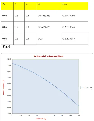
Fig. I shows the behaviour of working vacation queue length. It is clear from the graph that if service rate 1 increases then working vacation queue length is decreases.

[image:6.595.125.490.232.699.2]

Fig. II shows the behaviour of working vacation queue length. It is clear from the graph that if arrival rate  is increases then queue length is also increases.

Table I

P01   A Lqwv

0.06 0.1 0.3 0.08333333 0.04413793

0.06 0.2 0.3 0.16666667 0.23310346

0.06 0.3 0.3 0.25 0.89839085

Fig.-I

P

01







2

a

L

qwv

0.06

0.1

0.4

0.4

0.0625

0.02648157

0.06

0.1

0.5

0.4

0.05

0.018678107

0.06

0.1

0.6

0.4

0.041666667

0.014359822

0.06

0.1

0.7

0.4

0.035714286

0.011639526

0.06

0.1

0.8

0.4

0.03125

0.009775656

Fig.-II

It is clear from the Fig. -I that if the arrival rate is increases than queue length is also increases. Also From Fig – II, it is clear that if the service rate is increases than queue length decreases.

R

EFERENCES

[1] Ashok Kumar , “Application of Markovian process to queueing with cost Function PhD thesis, KU, Kurukshetra ” 1979 [2] Takagi H, “Mean message wasting time in asymmetric polling system Elsevier science publishers BV (North Holland)1990 [3] Chaudhary M.L and G C O “The queuing system M/GB/1 and its ramifications operation research-6” pp. 56-60.

[4] Ahmed M.M.S “Multi-channel bi-level heterogeneous servers, bulk arrivals queueing system with Erlangian service time”. Mathematical & computational applications, vol. 12 pp. 97-105. 2007