Network Simulation Methods of free convective flow from a vertical cone in the presence of non uniform surface heat flux

NETWORK SIMULATION METHODS OF FREE CONVECTIVE

FLOW FROM A VERTICAL CONE IN THE PRESENCE OF

NON-UNIFORM SURFACE HEAT FLUX

Immanuel Y1_{, Bapuji Pullepu}2 _{and Selva Rani M}2

1_{Department of Mathematics, Sathyabama University, Chennai, India}

2_{Department of Mathematics, SRM Institute of Science and Technology University, Kattan Kulathur, India}

E-Mail: [email protected]

ABSTRACT

Unsteady laminar free convection flow past a vertical cone with non-uniform surface heat flux

( )

m w

q x



ax

varying as a power function of the distance from the apex of the cone ( x = 0 ) under viscous dissipation effect is presented here. Here

m

is the exponent in power law variation of the surface heat flux and a is a constant. The unsteady, coupled and

non-linear dimensionless partial differential governing equations of the flow are solved using a Network Simulation Method. The effect of viscous dissipation



with various parameters Prandtl number

Pr

, and the exponent

m

_{for the} velocity and temperature profiles have been studied and are analyzed graphically. The local as well as average skin-friction and Nusselt number are also analyzed graphically. The present results are compared with available results in literature and are found to be in excellent agreement.

Keywords: finite difference method, heat transfer, laminar free convection, NSM, PSPICE, viscous dissipation, vertical cone.

INTRODUCTION

When a heated surface is in contact with the fluid, the result of temperature difference causes buoyancy force which induces natural convection heat transfer. This type of natural convection flows under the influence of gravitational force which occurs frequently in nature as well as in science and engineering applications. Hence they have been investigated extensively. The applications include, for example, the cooling of the core of a nuclear reactor in the case of a pump, or power failures and cooling of electric components. The basic solution of thermal convection from a heated or cooled surface due to suction or injection has numerous practical applications ranging from the cooling of manufactured products to the local weather forecasting level.

Merk and Prince[1-2] developed the general relations for similar solutions on isothermal axi-symmetric forms and showed that the vertical cone has such a solution. Eventhough numerous authors have investigated laminar free convection for the two-dimensional situation; this paper is concerned primarily with results for axi-symmetric flows. Approximate boundary-layer techniques were utilized to arrive at an expression for the dimensionless heat transfer. Hering [3] has obtained a number of similarity solutions for cones with prescribed wall temperature being a power function of the distance from the apex along the generator.

Heat flux applications are mainly being used in industries, engineering and science fields. Heat flux sensors can be used in industrial measurement and control systems. Detection fouling, Monitoring of furnaces and Flare monitoring are some of the applications of heat flux. Use of heat flux sensors can be lead to improvements in efficiency, system safety and modelling

The laminar free convection from a right circular cone with prescribed uniform heat flux conditions for all Prandtl numbers and expressions for both wall skin friction and wall temperature distributions at Pr →∞ were studied and similarity solutions are presented by Lin [4]. Hasan and Mujumdar[5] studied the free convective flow of a vertical cone with double diffusion effects under uniform flux condition. Watanabe [6] studied the effects of suction or injection on steady, free convection from a vertical cone with constant wall temperature condition. Chen et al.[7] studied the flows and heat transfer

characteristics of laminar free convection in boundary layer flows from horizontal, inclined and vertical plates with variable wall temperature and heat flux.Kafoussias [8] studied the effects of mass transfer on the laminar free convective flow past a vertical cone surface embedded in an infinite, incompressible and viscous fluid. Vajravelu and Nayfeh [9] analysed the convection flow and heat transfer in a viscous heat generating fluid near a cone and wedge with variable surface temperature and internal heat generation or absorption. The governing flow and heat transfer equations are solved numerically by using a variable order, variable step size finite-difference method. Yih[10] studied numerically in saturated porous media combined heat and mass transfer effects over a full cone with uniform wall temperature/concentration or heat/mass flux and for truncated cone with non-uniform wall temperature/variable wall concentration or variable heat/variable mass flux using the Keller box implicit difference method. Soundalgekar [11] studied about the free convective flow past a semi-infinite inclined plate for a viscous dissipative fluid. Bapuji et al. [12] studied the

the problem with non uniform surface heat flux including MHD with semi vertical angle.

The irreversible process by means of which the work is done by a fluid on adjacent layers due to the action of shear forces transformed into heat is defined as viscous dissipation. The effect of viscous dissipation in natural convection is appreciable when the induced kinetic energy becomes appreciable when compared to the amount of heat transferred. This occurs when either the equivalent body force is large or when the convection region is extensive. The effect of the viscous dissipation on heat transfer is significant, especially for high-velocity flows, for highly viscous flows even at moderate velocities, and for fluids with a moderate Prandtl number and moderate velocities with small wall to fluid temperature difference or with low wall heat fluxes and flowing through micro channels. Viscous dissipation occurs in natural convection in natural devices. Such dissipation effects may also be observed in the presence of strong gravitational fields and in processes wherein the scale of the process is very large, e.g., on large planets, in large masses of a gas in space and in geological processes, and in fluids internal to various bodies. Viscous mechanical dissipation effects are usually characterized by the Eckert number. Viscous dissipation effects can be measured by using an independent parameter called dissipation number. Taking this into account, viscous dissipative heat is included in the energy equation. The heat due to viscous dissipation in the energy equation is very small and is usually neglected. However, if the gravitational force is intensive or if the Prandtl number of the fluid is very high, the viscous dissipative effects cannot be neglected.

Genhart[14] was the first to study free convective flows over a vertical flat plate subject to isothermal and uniform flux surface conditions by an approximate method and also defined the non-dimensional dissipation parameter, Viscous dissipation is considered for vertical surfaces subject to both isothermal and uniform flux surface conditions using perturbation method. Kishore et al.[15] studied the thermal radiation and viscous

dissipation effects on the transient laminar free convection flow past a vertical cone with non-uniform surface temperature in the presence of a magnetic field.Mohiddin [16] studied the free convective flow past a vertical cone with vertical surface condition in the presence of viscous dissipation with radiation, MHD and mass transfer effects. Rishi et al.[17] studied the effect of Viscous dissipation on

natural convection heat and mass transfer from vertical cone in a non-newtonian fluid saturated with non-darcy porous medium. Palani el al. [18] examined the combined

effect of the magnetic field and viscous dissipation on a free convection flow of a compressible, viscous, and electrically conducting fluid past a semi-infinite vertical cone subjected to a variable surface heat flux. The system of dimensionless governing equations is solved by the finite difference method.

NSM simulates the behaviour of unsteady electric circuits by means of resistors, capacitors and non–linear devices that seek to resemble thermal systems governed by unsteady linear or non–linear equations. Electrical,

Thermal motion analogy provides a network model that is solved by means of a very common program used to simulate electrical circuits, Pspice[19]. NSM yields the ordinary differential equations the basis ones for implementing standard electrical network model for an elemental control volume from the partial differential equations that define the mathematical model of physical process and by means of spatial discretization Rektorys[20]. Alhama and Campo [21] represents the relation between NSM and heat transfer.

Alhama el al. [22] studied numerical solution of

the heat conduction equation with the electro thermal analogy and the code PSPICE. Zueco [23] studied for dissipative fluid, free convective flow past a vertical plate with constant heat flux using NSM. Zueco [24] studied the unsteady free convection in an infinite vertical parallel-plate channel with a viscous dissipative fluid and in the presence of buoyancy forces with constant thermal properties and subject to boundary conditions of the third kind, by means of the numerical Network Simulation Method. Zueco [25] developed a suitable network model to model the equations of the unsteady problem (MHD free convection flow past a semi-infinite vertical porous plate), with the fluid considered non-gray (absorption coefficient dependent on wave length), and study the effects of thermal radiation, viscous dissipation, suction / injection and magnetic field. Beg et al.[26] studied the

unsteady magnetohydrodynamic viscous Hartmann– Couette laminar flow and heat transfer in a Darcian porous medium intercalated between parallel plates, under a constant pressure gradient presence. Viscous dissipation, Joule heating, Hall current and ion slip current effects are included as is lateral mass flux at both plates. Unsteady MHD heat transfer in a semi-infinite porous medium with thermal radiation flux using network simulation method was studied by Beg et al.[ [27]. The steady, laminar

axisymmetric convective heat and mass transfer in boundary layer flow over a vertical thin cylindrical configuration in the presence of significant surface heat and mass flux are studied theoretically and numerically by Zueco el al.[28].

The objective of the present paper is to study unsteady free convective flow from a vertical cone with viscous dissipation and non uniform surface heat flux using a new method called the Network Simulation Method and it has not received any attention in the literature. The governing boundary layer equations are transformed into ordinary differential equations and are solved using the code PSPICE. In order to check the accuracy of the numerical results, the present results are compared with the available results of Palani and Kim [29], Hossain and Paul [30], Pop and Watnabe [31] and are found to be in excellent agreement.

Formulation of the problem

negligible. It is also assumed that the cone surface and the surrounding fluid which is at rest are at the same temperature

T

_



. Then at time

t

 

0

, it is assumed that heat is supplied from cone surface to the fluid at the rate

( )

m w

q x



ax

and it is maintained at this value with m being a constant.

Figure-1. Physical model of the coordinate system.

The co- ordinate system is chosen (as shown in Figure-1) such that x measures the distance along surface of the cone from the apex(x0)and y measures the distance normally outward. Here r x( )is the local radius of

the cone. The fluid properties are assumed to be constant except for density variations which induce buoyancy force and it plays vital role in free convection. The governing boundary layer equations of continuity, momentum, and energy under Boussinesq approximation are as follows:

Equation of continuity:

 

ur

 

vr 0

x y

 _  _

  (1)

Equation of momentum:

2 2

cos ( )

u u u u

u v g T T

t x y     y

 _  _  _{   } 



    (2)

Equation of energy:

2 2

2

p

T T T T u

u v

t x y y C y

                  _{ } 

      (3)

The initial and boundary conditions are

for all and ( )

0: 0, 0, at 0

at 0

0, as

0:

0,

0,

0,

w

x y

q x T

t u v y

y k

x

u T T y

t

u

v

T

T

u

T

T

                 











_{ }









_{ }

(4)

where

u

and

v

are the velocity components along

x

and

y

axes,

T



is the fluid temperature,

t



is the time, g is the acceleration due to gravity,

(

sin )

r



x



is the local radius of the cone,

q

_wis the uniform wall heat flux per unit area,



is the density of the fluid,

C

_Pis the specific heat at constant pressure,

k

is the thermal conductivity of the fluid,



is the thermal diffusivity,



is the thermal expansion coefficient, and



is the kinematic viscosity.

The physical quantities local skin-friction



_x

and local Nusselt number

Nu

_x are given, respectively by 0 y u y

x





    _ 

  (5)

0 y x w T x y Nu T T        _    

  (6)

where



is the dynamic viscosity. Also the average skin

friction L



is given by

2 0 0 2 L y L u x dx y L 



   _   

 

(7) Average heat transfer co-efficient

h

over cone surface is 0 2 2 0 y w T y k

h x dx

T T L L       _       



(8) The average Nusselt number

Nu

L is

0 2 0 L y w T y h L

Nu x dx

k L T T

L       _        



(9) Using the following non-dimensional quantities:

















 

 

1 5 '

1 2 2

5 5 5

2 1 ' ' 5 4 2

, , , where sin ,

, , ,

, Pr ,

( / )

( / ) cos

L

L L L

L w

w L

x y r

X Y Gr R r x

L L L

vL uL t

V Gr U Gr t Gr

L

T T

T Gr

q L k

g q L k L

and P

g L C



  where



is viscous dissipation

parameter as described in Gebhart [14] and

Gr

_Lis the grash of number.

Equations (1)-(3) are reduced to the following non dimensional form:

U R V R ₀

X Y

 _  _

  (11)

2 2

U U U U

U V T

t X Y Y

 _  _  _{ } 

    (12)

2 2

2

1 P r

T T T T U

U V

t X Y Y  Y

 _  _  _   

  

       (13)

Where

Pr

_{is the Prandtl number and}

R

is the

dimensionless radius of the cone. The corresponding non-dimensional initial and

boundary conditions are

0 : 0 , 0 , 0 f o r a l l a n d

0 : 0 , 0 , a t 0

0 , 0 a t 0

0 , 0 a t

m

t U V T x y

T

t U V X Y

Y

U T X

U T Y

   



     



  

   

(14)

Local skin-friction



_X and local Nusselt number

X

Nu

in non-dimensional quantities are

3 5

0

X L

Y U G r

Y







 

 _{ }



  (15)

1 1

5 0

.

m

X L

Y

X

N u G r

T



 

(16)

Average skin-friction



and average Nusselt number

Nu

in non-dimensional quantities are

1 3 5

0 0

2 L ,

Y

U

G r X d X

Y 





 

 _{ }



 



(17)

1

1 1

5 0

2 .

0 m L

Y

X

N u G r d X

T









(18)

Solution procedure

The governing partial differential equations (11)-(13) which are unsteady, coupled and non-linear with initial and boundary conditions (14) are solved using a new method called the network simulation method.

The network simulation method is a numerical technique for solving nonlinear heat conduction equations whose accuracy, efficiency and reliability have already been proven in numerous linear and nonlinear direct

problems in heat transfer engineering [20 - 28]. NSM is based on the classical electro –thermal analogy between thermal and electrical variables. Electrical and thermal systems are said to be analogous if they are formulated in the same domain with similar equations and identical initial and boundary conditions. The model is elaborated in network through space, not temporal, discretization. In the NSM technique, discretization of the differential equations is founded on the finite difference formulation, where discretization of the spatial coordinates is necessary, while time remains a real continuous variable. Hence, the imminent advantage of this method of non mathematical manipulations in the discretization of the time coordinate is necessary for most of the numerical methods used currently, since the code does this work. This is an essential difference between the most classic methods and the NSM.

Two circuits (Figures 1a and 1b) are developed for each non-dimensional boundary-layer equation.

Figure-1a. Network model of the control volume-momentum equation.

Figure-1b. Network model of the control volume-energy equation.

medium and boundary conditions and added by means of special electrical devices. The entire network model, including the devices associated with the boundary conditions is designed. A few programming rules are needed since not many devices form the network, solved by the numerical computer code Pspice [19] and the graph solution can be obtained by means the Probe software of Pspice. This code is imposed and adjusted continuously automatically for the time-step to reach a convergent solution in each iteration, according to the given stability and convergence requirements.

To solve the set of non-linear differential equation (11) – (13) subject to boundary condition (14) the NSM has been applied. The finite-difference differential equations resulting from dimensionless continuity, momentum balance, energy balance and mass balance equations are





    , , , , , )

– / – / / 2

/ i / 2 0 (

i X j i X j i j i j Y ri j

U U X V V Y

U X

        

   (19)













 





  , , , , , , , , , , , , / – /

– – / / 2

– / / 2

i j i j i X j i X j i j i j Y i j Y i j Y i j

i j i j Y i j

Y d U d t Y U U U X

V U U U U Y

U U Y Y T

                       (20)













 





 









, , , , , , , , , , , , , 2

Pr / Pr – /

Pr – – / / 2

– / / 2 Pr – /

i j i j i X j i X j i j i j Y i j Y i j Y i j i j i j Y i X j i X j

Y dT dt Y U T T X

V T T T T Y

T T Y  U U Y

                     (21)

In Equations. (20) and (21) all the terms can be treated as a current. Therefore implementing Kirchhoff’s law for electrical currents from circuit theory, the network model is obtained. To introduce the boundary conditions, voltage sources are employed to simulate constant values of velocity and temperature.

The NSM technique begins with the design of the network model of the element cell, following which we incorporate the boundary conditions. The following currents are defined

Momentum balance





 





 









, , , , , , , , , , , , , , , , , , , , , , , ,

– / / 2

– / / 2

– /

– /

U i j Y i j Y i j U i j Y i j i j Y U T i j i j

U x i j i j i X j i X j U y i j i j i j Y i j Y

U t i j i j

j U U Y

U U Y

j Y T

j Y U U U X

j V U U

j Y d U t

j d                             (22)

where

j

_{U i j, ,} _Y

and

j

_{U i j, ,} _Y are the currents

that leave and enter the cell for the friction term of U and are implemented by means two resistances

R

_{U i j, ,} _Y of

values “



Y

/ 2

”;

j

_{UT i j, ,} is the current due to the

buoyancy term and

j

_{Ux i j, ,}

and

j

_{Uy i j, ,} are the currents due to the inertia terms of U and V, respectively and are implemented by means of voltage control current generators

G

_{U, , , , i j}

G

_U, _{x i j, , ,}

G

_U, _{y i j, ,} . while

j

Ut i j, , is the transitory term and is implemented by means one capacitor of value

C

_{U i j, ,}

 

Y

, connected to the centre of each cell.

ii) Energy equation





, , , , , , , , , , , , , , , , , , , , , 2 , , , ,

( ) / ( / 2 )

( ) / ( / 2 )

P r ( T - T ) /

– )

P r /

/ (

T x i j i j i X j i X j

T y i j i

T i j Y i j i j Y

T i j Y i j Y i j

T i j i X j i X

j i j Y i j Y

T t i j i j

j

J T T Y

J T

j Y U X

j P r V T T

j

T Y

J U U

Y P r d T d t

Y                         V V V V V V V V V V V V (23) where

j

_{T i j, ,} _Y

and

j

_{T i j, ,} _Y are the currents

that leave and enter the cell for the friction term of U and are implemented by means two resistances

R

_{T i j, ,} _Y of

values “



Y

/ 2

”;

j

_{T i j, ,} is the current due to the buoyancy term and

j

_{Tx i j, ,}

and

j

_{Ty i j, ,} are the currents due to the inertia terms of U and V, respectively and are implemented by means of voltage control current generators

G

_{T, , , ,} _{i j}

G

_T, _{x i j, , ,}

G

_T, _{y i j, ,} . while

j

Tt i j, , is the transitory term and is implemented by means one capacitor of value

C

_{T t i j, , ,}

 

Y

, connected to the centre of each cell.

A more rigorous step-by-step numerical analysis is described by Gonzalez-Fernandez and Alhama [24], Zueco [26].

The finite difference equation corresponding to equation (10) is













, , ,

, ,

– / 2

+ /

i j i X j i X j

i j i j Y

V U U Y X

U Y i X V

            (24)

Above Equations [(20) – (21)] can be written in the form of Kirchhoff’s law as

, , , , , , , ,

, , , , 0

U i j Y U i j Y U T i j U x i j

U y i j U t i j

j j j j

j j

      

 

 (25)

, , , , , , , , , , , , 0

T i j Y T i j Y T i j Tx i j Ty i j Tt i j

j _ j _ j j j j  (26)

The uniqueness of the temperature variable is also satisfied due to Kirchhoff voltage law.

Finally, to implement the velocity, temperature boundary conditions (at X = 0 and as

Y

 

) ground elements are employed. Constant current and constant voltage at Y = 0 are utilized to simulate the non-uniform

heat flux (

T

m

X

Y



_{ }



). As regards the initial condition,

the voltages U = T = 0 for

t



0

are applied to the two capacitors

C

_{U i j, ,}

and

C

_{T i j, ,} .

RESULTS AND DISCUSSIONS

[image:6.612.98.507.241.395.2]

In order to prove the accuracy of our numerical results, the present results in steady state at

X



1.0

obtained are compared with available results in literature. Numerical values of temperature

T

, local skin-friction



X, for different values of Prandtl number

Pr

are shown in Table-1.

Table-1. Comparison of steady state local skin-friction values at X = 1.0 with those of Palani [29].

Pr

Temperature Local skin friction

Results of [29] Present results Results of[29] Present results

T T



_X



_X

0.72 1.78840 _1.7864* 1.7796 1.22705 _1.2240* 1.2154

1 1.63454 1.6263 1.08262 1.0721

2 1.36477 1.3578 0.83155 0.8235

4 1.15169 1.1463 0.63878 0.6328

6 1.04708 1.0421 0.54736 0.5423

8 0.98801 0.9754 0.49040 0.4859

10 0.93158 0.9272 0.45021 0.4460

100 0.56289 0.5604 0.18311 0.1813

*indicate the values obtained from Pop and Watanabe [31]

and that are compared with the results of [18] in steady state. In addition, the local skin-friction



Xand the local Nusselt number

Nu

_Xfor different values of Prandtl

number, when heat flux gradient

m



0.5

at

X



1.0

in steady state, are compared with the results of [11] in Table 2.

Table-2. Comparison of steady state local Nusselt number values at X = 1.0 with those of Hossain and Paul [30] for different values of Pr when m = 0.5 and suction is zero.

Pr

Local Skin friction Local Nusselt number Results of [30] Present results Results of [30] Present results

''

0

(0)

F



X

/

Gr

_L3/5

1/



0

(0)

Nu

X

/

Gr

L1/5

0.01 5.1345 5.1155 0.14633 0.1458

0.05 2.93993 2.9297 0.26212 0.2630

0.1 2.29051 2.2838 0.33174 0.3324

[image:7.612.143.537.58.425.2]

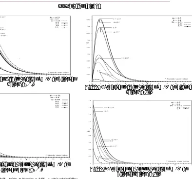
Figure 2: Transient velocity profile at X= 1.0 for different values of ‘



’.

Figure 3: Transient temperature profile at X= 1.0 for different values of ‘



’.

It is noticed from Figures 2 and 3 the transient velocity and temperature profiles are plotted at

X



1.0

for various values of



with

Pr 0.71



and

m



0.5

, the steady-state velocity increases with increasing viscous dissipation parameter



. It is evident that the temperature also increases with increasing viscous dissipative heating

[image:7.612.73.302.59.405.2]



. i.e. With a positive rise in



, there is a increase in velocity close to the cone surface, With an increase in



the time taken to attain the steady state also increased. The effect of viscous dissipation on flow field is to increase the energy, yielding a greater fluid temperature and as a consequence greater buoyancy force. The increase in the buoyancy force due to an increase in the dissipation parameter enhances the temperature. i.e The temperature in the boundary layer is elevated with a rise in



. Unlike the velocity response, the temperature profiles are all monotonic decays from the cone surface. The thermal boundary layer thickness reduces with decreasing



.

Figure 4: Transient velocity profile at X= 1.0 for different values of ‘Pr’.

Figure 5: Transient temperature profile at X= 1.0 for different values of ‘Pr’.

It also follows from Figures 4 and 5 transient velocity and temperature profiles are plotted at

X



1.0

for various values of Pr with

m



0.5

and





0.1

. Viscous force increases and thermal diffusivity reduces with increasing

Pr

, causes a reduction in the velocity and temperature. It is also noticed that the time taken to reach steady state increases and thermal boundary layer thickness reduces with increasing

Pr

. Also the momentum boundary layer thickness increases with the increase of

Pr

. Physically, it is possible because fluids with high Prandtl number have high viscosity and hence move slowly.

[image:7.612.321.539.186.415.2] [image:7.612.321.537.569.712.2]

[image:8.612.78.296.83.253.2]

Figure 7: Transient temperature profile at X= 1.0 for different values of ‘m’.

In Figures 6 and 7 transient velocity and temperature profiles are shown at

X



1.0

for various values of m with

Pr 0.71



and





0.1

. Impulsive forces are reduced along the surface of the cone near the vertex for increasing values of

m

(i.e. the gradient of heat flux along the cone near the apex reduces with the increasing values of

m

). Due to this, the difference between temporal maximum values and steady state values reduce. It is also observed that as

m

increases, velocity and temperature reduces and the time taken to reach steady state value increases.

[image:8.612.321.529.118.250.2]

The study of the effects of the parameters on local as well as the average skin-friction, and the rate of heat transfer is more important in heat transfer problems. In Figures 8-13 the local skin friction



_X and local Nusselt number

Nu

_X at various positions on the surface of the cone (X = 0.25 and 0.75) in the transient period are shown. The local skin friction



_X distribution for various values of

Pr

when





0.1

and

m



0.5

is shown in Figure-8. It is evident that the local wall shear stress decreases with increasing

Pr

because the flow velocity decreases as shown in Figure-4.

Figure 8: Local skin friction at X= 0.25 and 0.75 for different values of ‘Pr’ in transient state.

In transient period initially local skin friction almost constant throughout the surface and gradually

increases with time along the surface until it reaches steady state.

Figure 9: Local Nusselt number at X= 0.25 and 0.75 for different values of ‘Pr’ in transient state.

Figure-9 indicates the local Nusselt number

X

[image:8.612.322.540.339.487.2]

Nu

increases with increasing

Pr

and these effects gradually increase in the transient period with increasing the distance along the surface of the cone from the cone vertex along the surface of the cone.

Figure 10: Local skin friction at X= 0.25 and 0.75 for different values of ‘



’ in transient state.

[image:8.612.81.298.554.701.2]

Figure 11: Local Nusselt number at X= 0.25 and 0.75 for different values of ‘



’ in transient state.

[image:9.612.79.296.75.239.2]

Figure-11 depicts, an increase in the viscous dissipative heating leads to a reduction in the local Nusselt number

Nu

_X. i.e with a substantial increase in



a strong decrease in the surface heat transfer rate.

Figure 12: Local skin friction at X= 0.25 and 0.75 for different values of ‘m’ in transient state.

[image:9.612.326.534.182.325.2]

In addition from Figure-12. it is evident that with increasing

m

with

Pr

= 0.71and



=0.1, the local skin friction



_X decreases because the velocity gradient near the surface of the cone decreases.

Figure 13: Local Nusselt number at X= 0.25 and 0.75 for different values of ‘m’ in transient state.

Figure-13 shows that, with increasing

m

, the Nusselt number

Nu

_X increases, but the trend is slowly changed and reversed as distance increases along the surface from apex. i.e. near the leading edge, it decreases.

The average values of the skin friction and Nusselt number are given in Figures 14-19.

Figure 14: Average Skin friction for different values of ‘Pr’ in transient state.

Figure-14 reveals the average skin friction



decreases with increasing Prandtl number with



=0.1 and

m

=0.5.

Figure 15: Average Nusselt number for different values of ‘m in transient state.

We observe from Figure-15 the average Nusselt number also decreases with increasing values of

Pr

with

[image:9.612.79.294.329.489.2]



=0.1 and

m

=0.5.

[image:9.612.321.531.380.532.2] [image:9.612.82.292.564.716.2] [image:9.612.323.535.592.714.2]

Figure-16 shows an increase in



with

Pr

=0.71,

m

=0.5 the viscous dissipative heating leads to an increase in the average skin friction



.

Figure 17: Average Nusselt number for different values of ‘



in transient state.

In Figure-17 it also follows that the average Nusselt number

Nu

decreases with increasing viscous dissipation parameter



with

Pr

=0.71,

m

=0.5. The average Nusselt numbers are higher at the initial stage than at subsequent levels. Within a short time interval, the average Nusselt number is constant at each level of various parameters. This shows that heat conduction plays the major role at the initial stage. The average Nusselt number decreases with increasing dissipation parameter



.

Figure 18: Average skin friction for different values of ‘



in transient state.

Figure-18 indicates that average skin friction



decreases with increasing

m

for

Pr

=0.71and



=0.1 because the velocity gradient near the cone surface decreases. i.e. the average skin friction



increases with time and asymptotically reaches a constant value.

Figure 19: Average Nusselt number for different values of ‘m’in transient state.

Figure-19 shows that in the initial period, the average Nusselt number

Nu

does not change as

m

varies. This implies that, initially, heat transfer occurs only by heat conduction. In the initial period of convection, the average Nusselt number

Nu

slightly decreases and then increases with increasing

m

for

Pr

=0.71and



=0.1. CONCLUSIONS

The time taken to reach steady state decreases with decreasing values of

Pr

,

m

and



The velocity and temperature decreases with lower viscous dissipation



and increases for the lower values of the controlling parameters

Pr

and

m

.

The momentum and thermal boundary layers become thin for higher values of

m

and lower values of



. The momentum boundary layer becomes thick and thermal boundary layer becomes thin for higher values of

Pr

.

The local wall shear stress



_X increases for lower values

Pr

,

m

and higher values of



.

The local Nusselt number

Nu

_X decreases for smaller values of

Pr

,

m

and larger values of



.

The average skin-friction



decreases for smaller values



, and higher values of m and

Pr

.

The average Nusselt number

N

_u increases for lower values of



and higher values of

Pr

.

The effect of m on the average Nusselt number

u

N

is almost negligible. i.e. the average Nusselt number

[image:10.612.318.537.79.246.2] [image:10.612.75.298.133.275.2] [image:10.612.79.296.412.554.2]

NOMENCLATURE A Constant

0

(0)

F



Local skin friction in Hossain and Paul [30]

grashof number

acceleration due to gravity

ms

2

h

average heat transfer coefficient over surface _Wm-2_K-1 thermal conductivity Wm-1_K-1

reference length m

m

exponent in power law variation in surface _temperature

local Nesselt number

average Nusselt number

non-dimensional local Nesselt number non-dimensional average Nusselt number prandtl number

uniform wall heat flux per unit area

wm

2

dimensionless local radius of the cone local radius of the cone m

temperature

K

0

dimensionless temperature time s

dimensionless time

dimensionless velocity in X- direction velocity component in x- direction ms-1 dimensionless velocity in Y- direction velocity component in y- direction ms-1 dimensionless spatial co-ordinate

spatial co-ordinate along cone generator

m

dimensionless spatial co-ordinate along the normal to the cone generator

spatial co-ordinate along the normal to the cone generator

m

GREEK SYMBOLS

thermal diffusivity

m

2

s

1

volumetric thermal expansion 0

k

1

dimensionless time-step

Dimensionless finite difference grid size in X- direction-

Dimensionless finite difference grid size in Y- direction

Semi vertical angle of the cone

0

1/



(0)

Local Nusselt number in Hossain and Paul [30]



_{density kg} 3

m

dynamic viscosity kg

m

1

s

1



kinematic viscosity

m

2

s

1

local skin-friction

X



dimensionless local skin-friction

L



average skin-friction



dimensionless average skin-friction

SUBSCRIPTS

Condition on the wall Free stream condition

i associated with i nodal point J associated with j nodal point

REFERENCES

[1] Merk HJ, Prins JA.1953. Thermal convection laminar boundary layer I. Appl. Sci Res. 4: 11-24.

[2] Merk HJ, Prins JA.1953. Thermal convection laminar boundary layer II. Appl. Sci Res. 4: 195-206.

[3] Hering RG, Grosh RJ. 1962. Laminar free convection from a non iso- thermal cone, Int. J. Heat Mass Transfer. 5: 1059-1068.

[4] Lin FN. 1976. Laminar free convection from a vertical cone with uniform surface heat flux, Lett. Heat. Mass. Trans. 3: 49-58.

[5] Hasan M, Mujumdar AS. 1984. Coupled heat and mass transfer in natural convection under flux condition along a vertical cone, Int. Comm. Heat Mass Transfer. 11: 157-172.

[6] Watanabe T. 1991. Free convection boundary layer flow with uniform suction or injection over a cone, Acta Mech. 87: 1-9.

[7] Chen TS, Tien HC, Armaly BF. 1986. Natural convection on horizontal, inclined and vertical plates with variable surface temperature or heat flux, Int. J. Heat Mass Transfer. 29: 1465-1478.

[8] Kafoussias NG. 1992. Effects of mass transfer on free convective flow past a vertical isothermal cone surface. Int. J. Eng. Sci. 30(3): 273-281.

[9] Vajravelu K, Nayfeh J. 1992. Hydro magnetic convection at a cone and a Wedge, Int. Comm. Heat Mass Transfer. 19: 701-710.

[10]Yih KA. 1999. Coupled heat and mass transfer by free convection over a truncated cone in porous media: VWT/VWC/ or VHF/VMF, Acta Mech. 137: 83- 97. L

Gr

g

k

L

x

Nu



L

Nu



X

Nu

Nu

Pr

q

R

r

T



T

t



t

U

u

V

v

X

x

Y

y





t



X



Y







x







[11]Soundalgekar VM, Jaiswal BS, Uplekar AG, Takhar HS. 1999. Transient Free Convection Flow of Viscous Dissipative Fluid past a Semi-Infinite Inclined Plate, Appl. Mech. Eng. 4(2): 203-218.

[12]Bapuji Pullepu, Ekambavanan K, Pop I. 2008. Transient laminar free convection from vertical cone with non-uniform surface heat flux, Studia Univ.Babes-Bolyai Mathematica. L III(1): 75-99.

[13]Bapuji Pullepu, Chamkha AJ. 2009. Transient laminar MHD free convective flow past a vertical cone with non-uniform surface heat flux’, Nonlinear Anal. Model. Control. 14(4): 489-503.

[14]Gebhart B. 1962. Effects of viscous dissipation in natural convection, J. Fluid Mech. 14: 225-232.

[15]Kishore PM, Rajesh V, Vijayakumar Verma S. 2010. Viscoelastic buoyancy- driven MHD free convective heat and mass transfer past a vertical cone with thermal radiation and viscous dissipation effects, Int. J. Mathematics and Mechanics. 6(15): 67-87.

[16]Mohiddin SG, Vijayakumar Verma S, Iyengar NChSN. 2010. Radiation and mass transfer effects on MHD free convective flow past a vertical cone with variable surface conditions in the presence of viscous dissipation, Int. Elec. Eng. Math. Soc. 8: 22-37

[17]Rishi Raj kairi, Murthy PVSN. 2011. Effect of Viscous Dissipation on Natural Convection Heat and Mass Transfer from Vertical Cone in a Non-Newtonian Fluid Saturated Non-Darcy Porous Medium, Appl. Math. and Comput. 217(20): 8100-8114.

[18]Palani G, Ragavan A, Thandapani R E. 2013. Effect of viscous dissipation on an MHD free convective flow past a semi-infinite vertical cone with a variable surface heat flux. J. Appl. Mech. Tech. Phy. 54(6): 960-970

[19]Pspice, 6.0, /Microsim Corporation, 20, Fairbanks, Irine, California - 92718, 1994.

[20]Rektorys K. The method of discretization in time for PDE, D. Reidel Publishers, Dordrechet, The Netherlands, 1982.

[21]Alhama F, Gonzalez- Fernandez CF. 2002. Heat Transfer and the Network simulation method, NSM, Research signpost, Trivandrum. 35-58.

[22]Alhama F, Campo A, Zueco J. 2005. Numerical solution of the heat conduction equation with the electro – thermal analogy and the code PSPICE, Appl. Math. Comput. 162: 103-113.

[23]Zueco J. 2006. Numerical study of an unsteady free convective magneto hydrodynamics flow of a dissipative fluid along a vertical plate subject to a constant heat flux, Int. J. Eng. Sci. 44: 1380- 1393.

[24]Zueco J. 2006. Network method to study the transient heat transfer problem in a vertical channel with viscous dissipation, Int. Commun. Heat Mass. 33: 1079-87.

[25]Zueco J. 2007. Network simulation method applied to radiation and viscous dissipation effects on MHD unsteady free convection over vertical porous plate, Appl. Math. Model. 31: 2019-2033.

[26]Beg OA, Zueco J, Takhar HS. 2009. Unsteady magnetohydrodynamic Hartmann-Couette flow and heat transfer in a Darcian channel with Hall current, ionslip, viscous and Joule heating effects: Network numerical solutions, Commun. Nonlinear Sci. Numer. Simulat. 14: 1082–1097.

[27]Beg OA, Zueco J, Ghosh SK, Heidari Alireza. 2011. Unsteady MHD heat transfer in a semi – infinite porous medium with thermal radiation flux: Analytical Numerical Study, Adv. in Numer. Anal. 2011: 1-17.

[28]Zueco J, Beg OA, Takhar HS, Nath G. 2011. Network Simulation of Laminar Convective Heat and Mass Transfer over a Vertical Slender Cylinder with Uniform Surface Heat and Mass Flux, J. Appl. Fluid. Mech. 4(2): 13-23.

[29]Palani G, Kim KY. 2012. Influence of magnetic field and thermal radiation by natural convection past vertical cone subjected to variable surface heat flux. Appl. Math. Mech. 33(5): 605-620.

[30]Hossain MA, Paul SC. 2001. Free convection from a vertical permeable circular cone with non-uniform surface heat flux. Heat Mass Transfer. 37: 167-173