www.ijsrp.org
Estimation of confidence intervals for Multinomial
proportions of sparse contingency tables using Bayesian
methods
U. Sangeetha*, M. Subbiah**, M.R. Srinivasan***
*
Department of Management Studies, SSN College of Engineering, Chennai.
**
Department of Mathematics, L. N. Government College, Ponneri.
***
Department of Statistics, University of Madras, Chennai.
Abstract - Multinomial distribution, widely used in applications with discrete data, witnessed varieties of competing intervals from frequentist to Bayesian methods, still prove to be interesting in the case of zero counts or sparse contingency tables. The methods commonly recommended in both approaches are considered based on its influence of zero counts, polarizing cell counts, and aberrations. The inference based on comparative study shows that Bayesian approach, with an appropriate prior could be a good choice in dealing with a sparse data set without any imputation for zero values.
Index Terms:Bayesian inference, Coverage probabilities, Dirichlet distributions, Multinomial distributions, sparse data
.
I.INTRODUCTION
he cell of contingency table contains frequency of outcomes of categorical response variables and its number denotes the dimension and size is determined by number of categories related to each of the variable. Generally, inferential methods for categorical data assume multinomial or Poisson sampling models. The observed counts {ni; i=1,2,…,k} could be considered as k levels of a single categorical variable or for k=IJ cells of a two way categorical variables with levels I and J. Agresti (1992) has explained the different sampling k models and in particular, the present work is based on the multinomial distribution ( ,{ 1, 2,…, k}) Maximum likelihood estimates (MLE) of cell probabilities can be derived easily as sample cell proportions but interval estimation of multinomial probabilities too has drawn then active attention.
The impact of sparseness provides an ample scope to have a comparative study among these methods as well as Bayesian procedures. Agresti and Yana (1987) have stated that the asymptotic approximations may be quite poor for sparse table, even for a large N. Further Szyda et al (2008) observed that sparseness could occur even when k is relatively large. Subbiah and Srinivasan (2008) have studied the nature of sparseness in a 2x2 table based on a summary measure. Also, recent developments have favored Bayesian approaches as more suitable methods to handle sparseness as compared to three standard recommendations while handling sparse or zero counts (Agresti, 1992, Subbiah et al 2008).
The objective of this paper is to draw comparisons that include Bayesian approach with non-informative priors for underlying parameters. Study envisages use of typical 2x2 data sets in the literature and a large contingency table (Szyda etal, 2008). Frequentist property of coverage probabilities for Bayesian approach have also been studied and compared with the available results of classical approaches using recent computational tools. The following section provides a comprehensive list of active methods in the literature considered for comparison of confidence intervals for multinomial proportions.
II. CONFIDENCE INTERVALS FOR MULTINOMIAL PROPORTIONS
In the case of Bayesian inference, Dirichlet distribution is the widely used and recommended conjugate prior distribution for the multinomial probability parameters (Gelman et al, 2000). However, to obtain posterior distribution, a relationship between Ga mma distribution and Dirichlet distribution has been used and presented as
i a a ( i,1) , =∑i=1k i a a ( ,1) ere =∑ki=1 i
Then ( 1, 2,…, k) iric le 1, 2,…, k .
With a proper choice of hyper parameters { } a complete Bayesian scheme can be implemented. However, recent advances in the Monte Carlo simulations, posterior summaries can directly be obtained from simulating Dirichlet distribution. The typical scheme (MD) is
ni ul ino ial ( ,{ 1, 2,…, k})
www.ijsrp.org
iric le 1 n1 ,…, k nk
Setting ( ) will yield a uniform density and Tuyl et al (2009) have favoured this choice as a better non informative
prior for { }
=1 k
Further, a simulation study has been carried out to compare the performance of the intervals in terms of repeated experiments. Bayesian estimates obtained from incorporating objective priors might require such a test based on frequentist approach. Agresti and Min (2005) have attempted this in evaluating the Bayesian confidence intervals for binomial proportions. The corresponding procedure for multinomial proportions includes following steps
1) Consider any data set with cell count {n1,n2,…….nk}
2) Compute its MLE p = {ni/N} and assume p as population parameter 3) Simulate Multinomial(N, p) for L times
4) Obtain confidence interval using the required methods
5) Coverage Probability = (Number of intervals in (iv) that include p) / L
Similar attempts have been made for classical approaches or Bootstrap intervals in literature that are cited earlier in this paper. This work includes Bayesian methods by considering contingency tables with non-zero but low counts and has an appreciable distance between the counts. However for comparison purpose other standard procedures such as QH-Quesenberry and Hurst (1964), GM-Goodman (1965), FS- Fitzpatrick and Scott (1987), SG- Sison and Glaz (1995) and methods due to central limit theorem (CLT) and its continuity corrected version (CLT-CC) have also been considered.
III. MOTIVATING DATA SETS
[image:2.612.67.501.406.467.2]If X and Y denote two categorical response variables, X with I categories and Y with J categories leading to k = IJ possible combinations that can be represented in a contingency or cross-classification table with cells contain frequency counts of outcomes for a sample. As a case of a hypothetical example, suppose that a clinical trial is undertaken to compare the effect of a new drug or other therapy with the current standard drug or therapy. Ignoring side effects and other complications, the response for each patient is assu ed o be si ply “success” or “failure.” For a single s and-alone experiment, the observed data can be shown in the following table:
Table 1: Hypothetical responses in one segment of a clinical trial
Response
Success Failure Total
Treatment a b m
Control b d n
Total r s N
Sparse tables often contain cells having zero counts and such cells are called empty cells. Contingency tables are referred to as sparse when many cells have small frequencies besides some of them being zeros too. It is extremely important to describe the location of zero cells in the 2 x 2 table, as the same is also crucial in studying the nature of sparsity and could affect the analysis. Sparsity is not restricted to the tables with smaller sample sizes alone but could also occur with large sample size due to high concentration of frequencies in certain cells and poor or none in other cells. The impact of sparsity is felt in estimation of summary measures like odds ratio, computational complexity and asymptotic approximations. Even for large contingency tables, due to the small sample size and the resulting sparseness of the data table, the asymptotic distributions of the tests may not be relied in hypothesis testing (Szyda et al 2008).
www.ijsrp.org Table 2: General description of the ten illustrative data sets
Data
No Source of data sets
Zero entries Positive
entries < 6 Range of table totals No of tables with nature of Sparseness
No % No % Min Max Mild Moderate Severe
I Kishore (2007) 5 18 4 14 0 17 3
II Agresti (1990) 7 35 9 45 5 6 5
III Smith et al (1995) 2 2 10 11 12 158 2
IV Sweeting et al (2004) 37 40 9 10 15 1128 19 2
V Sweeting et al (2004) 2 7 6 21 688 66153 1 1
VI Efron (1996) 16 10 43 26 0 48 3 2 1
VII Tian et al (2007) 48 25 45 23 25 2852 27 11 3
VIII Tian et al (2007) 67 35 27 14 25 2852 30 9 3
IX Cochran (1954) 4 25 3 19 17 40 1 3
X Warn et al (2002) 17 9 18 10 7 177 15 2
Apart from these ten 2 x 2 tables, another contingency table (Szyda et al 2008) has been considered whose size is 4 x 5 of which 12 cells (60%) are zero where as minimum and maximum among remaining non-zero cells are 5 and 66 respectively. This data illustrates the presence of more zeros and extreme non-zero counts with high range even in a large size tables. These observations among many such real time studies provide a notion for comparative study using relevant characteristics which are prevalent in data sets summarized in contingency tables.
IV. RESULTS
Bayesian data analysis can be referred to posterior inference given a fixed model and data and computation has been carried out in WinBUGS and R. However, sufficient search indicates non availability of classical methods in open sources and these methods are implemented using Macros in EXCEL except SG which is obtained through SAS.
Results from the computations include lower and upper limits of 95% confidence intervals calculated from the closed form classical methods. 2.5 and 97.5 percentiles from posterior samples are used to obtain lower and upper limits of Bayesian confidence intervals after a run of 50000 single MCMC chain with burn-in of initial 50% and convergence has also been monitored using kernel density. However, Table 3 provides results from one data set as an illustrative case and subsequently observations from the comparative analysis have been presented. This data set has as many characteristic as desired in explaining the performance of these procedures; especially, under sparseness, low non-zero counts and the impact on corresponding results.
The comparisons are based mainly on length of intervals (shorter or wider), aberrations; many studies have considered coverage probability as a tool for comparing performance of intervals. However, very limited or no studies have included Bayesian method in this comparison and this study has considered Bayesian MD procedure and compare with existing results. The data characteristics such as sparseness in terms of presence of zeros and low cell counts range of cell counts in a table and size of the table. Though computation tools become abundant in the present scenario, these procedures require a keen attention in the availability to the user community.
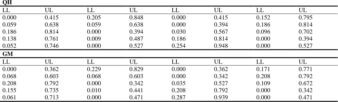
Table 3: Comparison of seven simultaneous confidence interval procedures with α = 0.05 for five different 2 x 2 tables QH
LL UL LL UL LL UL LL UL
0.000 0.415 0.205 0.848 0.000 0.415 0.152 0.795
0.059 0.638 0.059 0.638 0.000 0.394 0.186 0.814
0.186 0.814 0.000 0.394 0.030 0.567 0.096 0.702
0.138 0.761 0.009 0.487 0.186 0.814 0.000 0.394
0.052 0.746 0.000 0.527 0.254 0.948 0.000 0.527
GM
LL UL LL UL LL UL LL UL
0.000 0.362 0.229 0.829 0.000 0.362 0.171 0.771
0.068 0.603 0.068 0.603 0.000 0.342 0.208 0.792
0.208 0.792 0.000 0.342 0.035 0.527 0.109 0.672
0.155 0.735 0.010 0.441 0.208 0.792 0.000 0.342
[image:3.612.32.582.543.709.2]www.ijsrp.org CLT
LL UL LL UL LL UL LL UL
0.000 0.000 0.170 0.920 0.000 0.000 0.080 0.830
0a 0.562 0a 0.562 0.000 0.000 0.139 0.861
0.139 0.861 0.000 0.000 0a 0.435 0a 0.673
0.061 0.772 0a 0.283 0.139 0.861 0.000 0.000
0.104 0.580 0.000 0.000 0.288 1.141 0.000 0.000
CLT-CC
LL UL LL UL LL UL LL UL
0a 0a 0.125 0.875 0a 0a 0.034 0.784
0a 0.521 0a 0.521 0a 0a 0.098 0.819
0.098 0.819 0a 0a 0a 0.394 0a 0.632
0.020 0.730 0a 0.241 0.098 0.819 0a 0a
0a 0.641 0a 0a 0.216 1b 0a 0a
SG
LL UL LL UL LL UL LL UL
0.000 0.346 0.364 0.892 0.000 0.346 0.273 0.801
0.000 0.527 0.000 0.527 0.000 0.277 0.250 0.777
0.250 0.783 0.000 0.283 0.000 0.450 0.083 0.616
0.167 0.692 0.000 0.359 0.250 0.776 0.000 0.276
0.143 0.684 0.000 0.398 0.571 1.000 0.000 0.398
FS
LL UL LL UL LL UL LL UL
0a 0.089 0.456 0.635 0a 0.089 0.365 0.544
0.168 0.332 0.168 0.332 0a 0.082 0.418 0.582
0.418 0.582 0a 0.082 0.085 0.248 0.252 0.415
0.335 0.498 0.002 0.165 0.418 0.582 0a 0.082
0.146 0.426 0a 0.140 0.574 0.854 0a 0.140
MD
LL UL LL UL LL UL LL UL
0.002 0.226 0.228 0.710 0.002 0.235 0.179 0.645
0.078 0.487 0.077 0.487 0.002 0.218 0.212 0.679
0.209 0.676 0.002 0.221 0.044 0.402 0.119 0.550
0.165 0.619 0.017 0.320 0.211 0.677 0.002 0.219
0.067 0.562 0.003 0.303 0.267 0.813 0.003 0.307
a Lower limit is less than zero b Upper limit is greater than one
In terms of length of intervals for the data sets (I to X), SG (63%) and QH (31%) yield wider intervals compared to other methods. SG has the maximum length in most of the cases where range of cell counts are markedly as high as 6821. Even in such polarized tables, only small count cells have this property and QH produces long intervals for other cells of corresponding tables. Data set IV, VI, VII, VIII, and few tables of X can be considered as illustrative cases which exhibit this observation where the distance among the individual counts are notably high and more tables are available with the presence of zeros in different position of four cells. This property is apparent in the data set III in which all cell counts are non-zero counts except in two cells among the total of 88 cells (22 tables).
In the data set V, possibly a rare table with an extreme characteristic in that cell counts are too wider (10, 45870, 40, 66163) is available. MD provides a wider interval only in this case for the low counts and QH has shared this for other larger values and except this case, MD has not shown this property in any of the other tables considered for the comparisons that are presented here and other data sets with which this study has made extended comparisons.
www.ijsrp.org
In the case of shorter intervals, FS dominates uniformly in all the four cells of all data sets considered for the study; 72%, 95%, 60% and 94% of occasions are the supportive numerals for this property. In each case, CLT methods immediately succeed FS in this property but this may be due to its feature already mentioned and hence could be avoided from comparison. Surprisingly SG yie ld shorter intervals in two tables of the data set V where counts are extremely varying in nature (range 8632 and 66153). No other methods exhibit this property in any of cases considered for the comparative study.
It is observed that aberrations exist in three procedures due to CLT based methods and FS. But those cells cannot be identified with any particular characteristic of a cell like zero count. In the case of zero counts these methods will yield a degenerate case with lower and upper limits are same value. This feature is an obvious outcome of their mathematical forms. Also, a closer look of CLT indicates that the procedure will be resulted with a smoothing by the chi square value whenever cell counts are zero. This kind of smoothing would encourage the recommendation of Bayesian procedure as observed in Agresti (1992). Also, from Table 3 it can be observed that upper limit can also have estimates that are not possible for a proportion; in limits of CLT based intervals exceed one where as SG yields exactly one as upper limit where the observed proportion is quite nearer to one and as low as five.
Further nature of sparseness has been considered in understanding the performance of these methods in term of extreme lengths; three classifications of sparseness also demonstrate this behavior. QH and SG perform uniformly across these classifications and CLT based intervals provide wider intervals even in the case of mild sparse as well as all the four cells are with low counts. However, because FS dominates uniformly while comparing shorter intervals, nature of sparseness has not been considered in those cases.
The analysis schemes have been extended to a data set that has a 4 x 5 contingency table (Syzdaetal, 2008) with many zeros. Results have shown that no major changes in terms of longest interval are visible when compared to 2 x 2 tables. QH has dominated uniformly over all non zero cells in the table followed by SG and GM. However, unlike the case 2 x 2 table, this behavior does not distinguish between low or high non zero counts. Also, FS yields smaller intervals in all cases that may not be a required feature for an interval estimator. Bayesian method yields a better compromise estimates when compared to these methods with extreme values. The inevitable 0.0 as estimates for zero counts in the case of CLT methods are apparent for this data set too. But CLT-CC yields a negative lower limit for a case where the count is five. Hence when table size (k) or total counts (N) become large, the negative lower limit could appear in the case of cell counts over and above five.
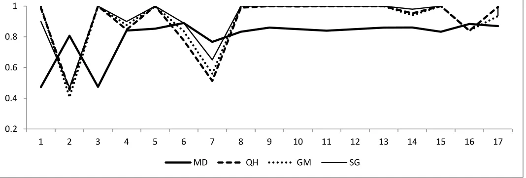
Also, the outcome of simulation studies indicate a consistent behavior of Bayesian confidence intervals when compared to classical approach though MD intervals are uniformly narrower than other counterparts and achieves coverage probability less than 0.95. Agresti and Coull (1998) have pointed out that such property can also be preferred in certain cases and very wider intervals which may tend to provide very high coverage probability in most of the cases. This attempt includes another data of size 1 x 7 (Quesenberry and Hurst,1964) that has been used almost in all similar studies that is beyond the data sets considered in this Section. Figure 1 presents the illustrative details of the consistent behavior of MD and the extreme performance of QH, GM, and SG; CLT methods and FS are not considered for this comparison based on their performance that is observed earlier.
Figure 1: A comparison of coverage probabilities for the nominal 95% QH, GM, SG and MD intervals for multinomial proportions
0.2 0.4 0.6 0.8 1
1 2 3 4 5 6 7 8 9 10 11 12 13 14 15 16 17
[image:5.612.39.573.465.646.2]www.ijsrp.org
All these data sets represent the varied feature of contingency tables so that methods can be compared for the performance of the methods. Extreme range of cell counts where classical methods are consistently closer to one whereas MD provides around 85% as its coverage probability in all such cases. From the figure it can be observed that there is a reversal tendency in the case of second set where cell counts are low and classical procedures have as low as 45%. Similar effect is also the case when cell counts are high but of notably apart from each other. Hence, in the absence of a perfect definition of sparseness in a general I x J tables, MD has a consistent behavior in terms of coverage probability though the numerical value is below the nominal value.
V. CONCLUSIONS
Multinomial proportions have found many applications and Burda et al (2008) have provided illustrative cases for multinomial discrete models. Lee et al (2011) have applied the methods for constructing confidence intervals for multinomial proportions to the design process of grain tracing and recall system. Kern (2006) has used a pig data to illustrate the Bayesian inference on multinomial probabilities. The present study has emphasized the need to understand, implement and compare the procedures in obtaining confidence intervals for multinomial proportions, especially when the data is sparse in nature.
In general, comparison and subsequent recommendation of any statistical procedures are based on their performance, wider availability to the users, computational issues, and aberrations. Further sparseness also plays an important role in deciding the procedure to be adopted. Agresti (1990) has stated that for sampling zeros, it is not sensible to use 0.0 as the best estimate of a probability. In view of this, classical methods, which yield 0.0 as estimator either because of its form or through auto corrections, need not be recommended if the data sets do have more zeros. Hence zero counts irrespective of other cell counts need a careful investigation in using an estimation method. Bayesian procedures even with a non informative prior yield estimates in such situations similar to its performance uniformly over 2 x 2 tables considered as a basic form in many categorical data studies.
Such similarity is consistently visible when the size of the table increases and range of the cell counts is relatively higher. However a classical method needs careful choice when k or N changes also when the cell counts are comparatively different. Further it may be easier in the present scenario to obtain a computation tool or mechanism, but still the availability of these classical methods is restricted to Wald type intervals. However, CLT based methods are not recommended when data is sparse irrespective of zero or non zero counts and size of the table.
Bayesian procedure has distinct advantages in obtaining the confidence limits without any aberrations; possessing acceptable frequentist coverage probabilities and practically important in computational flexibility and availability. It has been observed that exact inference plays important role in statistical inference of discrete data; however, for sparse data large sample chi-square statistics are often unrealistic (Agresti and Coull, 1998). More importantly, all of these conclusions are drawn for sparse data which is more realistic even for large contingency tables. Hence, this comparative study has emphasized the need to apply Bayesian methods with an objective prior for estimating multinomial proportions in categorical data with presence of zero or low cell counts and has an appreciable difference between the cell counts; in some cases the number of categories also plays a role to choose between methods. Bayesian methods have been identified as unified approach to handle varied situations of cell frequencies that would generally arise in the analyses of contingency tables and its applications.
REFERENCES [1] A. Agresti, Categorical Data Analysis. John Wiley & Sons, New York, 1990.
[2] A. Agresti, “A survey of exact inference for contingency tables”.Statistical Science. 1992. 7: 131 – 177.
[3] A. Agresti, and B.A. Coull, “Approxi a e is be er an “Exac ” for in erval es i a ion of bino ial propor ions”. The American Statistician. 1998. 52: 119 – 126. [4] A. Agresti, and Y. Min, “Frequentist performance of Bayesian confidence intervals for comparing proportions in 2 × 2 contingency tables”. Biometrics. 2005. 61:
515 – 523.
[5] A. Agresti, and M.C. Yang, “An empirical investigation of some effects of sparseness in contingency tables”. Computational Statistics & Data Analysis. 1987. 5: 9 – 21.
[6] L.D. Brown, T.T. Cai, and A. DasGupta, “Interval estimation for a binomial proportion”. Statistical Science. 2001. 16: 101 – 133.
[7] M. Burda, M. Harding, J. Hausman, “A Bayesian mixed logit-probit model for multinomial choice”. Journal of Econometrics. 2008. 147: 232 – 296.
[8] W.G. Cochran, “Some methods for strengthening e co on χ2 tests”. Biometrics. 1954. 4: 417 – 451.
[9] B. Efron, “Empirical Bayes methods for combining likelihoods”. Journal of American Statistical Association. 1996. 91: 538 – 565.
[10] S.P. Fitz, A. Scott, “Quick simultaneous confidence interval for multinomial proportions”. Journal of American Statistical Association. 1987. 82(399): 875 – 878.
[11] A. Gelman, J.B. Carlin, H.S. Stern, and D.B. Rubin, Bayesian Data Analysis: Chapman & Hall, London. 2000.
www.ijsrp.org
[13] L.A. Goodman, “On Simultaneous Confidence Intervals for Multinomial Proportions”. Technometrics. 1965. 7: 247 – 254.
[14] C.D. Hou, J. Chiang, J.J. Tai, “A family of simultaneous confidence intervals for multinomial proportions”. Computational Statistics & Data Analysis. 2003. 43: 29 – 45.
[15] J.C. Kern, “Pig Data and Bayesian Inference on Multinomial Probabilities”. Journal of Statistics Education 14. 2006.
http://www.amstat.org/publications/jse/v14n3/datasets.kern.html
[16] B.K. Kishore, “Statistical models for multi-centric trials and their applications”. Unpublished Ph.d Thesis, University of Madras. 2007.
[17] Lee, P.R. Armstrong, J.A. Thomasson, R. Sui, M. Casada, “Application of binomial and multinomial probability statistics to the sampling design process of a global grain tracing and recall system”. Food Control. 2009. 22: 1085 – 1094.
[18] M. Jhun, H.C. Jeong, “Applications of bootstrap methods for categorical data analysis”. Computational Statistics & Data Analysis. 2000. 35: 83 – 91.
[19] L.W. May, D.W. Johnson, “Constructing simultaneous confidence intervals for multinomial proportions”. Computer Methods and Programs in Biomedicine.
1997. 53: 153 – 162.
[20] C.P. Queensberry, D.C. Hurst, “Large Sample Simultaneous Confidence Intervals for Multinational Proportions”. Technometrics.1964. 6: 191 – 195.
[21] P.C. Sison, and J. Glaz, “Simultaneous Confidence Intervals and Sample Size Determination for Multinomial Proportions”. Journal of the American Statistical
Association. 1995. 90: 366 – 369.
[22] C.T. Smith, D.J. Spiegelhalter, and A. Thomas, “Bayesian approaches to random-effects meta-analysis: a comparative study”. Statistics in Medicine. 1995. 14: 2685 – 2699.
[23] M. Subbiah, and M.R. Srinivasan, “Classification of 2 x 2 sparse data with zero cells”. Statistics & Probability Letters. 2008. 78: 3212 – 321.
[24] M. Subbiah, B.K. Kishore, and M.R. Srinivasan, “Bayesian approach to multicentre sparse data”. Communications in Statistics - Simulation and Computation. 2008. 37: 687 – 696.
[25] J.M. Sweeting, J.A. Sutton, and C.P. Lambert, “What to add to nothing? Use and avoidance of continuity corrections in meta-analysis of sparse data”. Statistics in Medicine. 2004. 23: 1351 – 1375.
[26] J. Szyda, Z. Liu, D.M. Zaton, H. Wierzbicki, A. Rzasa, “Statistical aspects of genetic association testing in small samples, based on selective DNA pooling data in
the artic fox”. Journal of Applied Genetics. 2008. 49: 81 – 92.
[27] L. Tian, T. Cai, N. Piankov, P. Cremieux, and L. Wei, “ Effectively combining independent 2 x 2 tables for valid inference in meta analysis with all available data but no artificial continuity corrections for studies with zero events and its application to the analysis of rosiglitazone's cardiovascular disease related event data”. Harvard University: www.bepress.com/harvardbiostat/paper69. 2007.
[28] F. Tuyl, R. Gerlach, K. Mengersen, “Posterior predictive arguments in favor of the Bayes-Laplace prior as the consensus prior for binomial and multinomial parameters”. Bayesian Analysis. 2009. 4: 151 – 158.
[29] D.E. Warn, S.G. Thompson, and D.J. Spiegelhalter, “Bayesian random effects meta-analysis of trials with binary outcomes: methods for the absolute risk difference and relative risk scales”. Statistics in Medicine. 2002. 21: 1601 – 1623.
AUTHORS
First Author – U. Sangeetha, M.Sc., M.Phil. Department of Management Studies, SSN College of Engineering, Chennai.
Second Author – M. Subbiah, M.Sc., M.Phil., Ph.D. Department of Mathematics, L. N. Government College, Ponneri.
Third Author – M.R. Srinivasan, M.Sc., MBA., Ph.D. Department of Statistics, University of Madras, Chennai.