Convexity Preserving C
2
Rational Quadratic
Trigonometric Spline
Mridula Dube
*, Preeti Tiwari
** *Department of Mathematics and Computer Science, R. D. University, Jabalpur, India. **
Department of Mathematics, G.G.I.T.S., Jabalpur, India.
Abstract- A C2 rational quadratic trigonometric spline interpolation has been studied using two kinds of rational quadratic trigonometric splines. It is shown that under some natural conditions the solution of the problem exists and is unique. The necessary and sufficient condition that constrain the interpolant curves to be convex in the interpolating interval or subinterval are derived. approximation properties has been discussed and confirms the expected approximation order is h2.
Index Terms- Approximation, Constrained interpolation, Continuity, Convexity, Rational quadratic trigonometric spline, Shape parameter .
I. INTRODUCTION
uring the recent years rational parametric spline have gained widespread acceptance for use in computer aided geometric designs.They have been studied by several authors (see [1], [4], [8], [10]), with special emphasis on the shape preserving properties. In [1] Duan have presented the construction and shape preserving analysis of a new weighted rational cubic interpolation and its approximation. Trigonometric splines serves as an alternative for polynomial splines for solving many problems of interpolation and have been studied from application point of view (see [2], [3], [5], [6], [7], [9]). Trigonometric splines behave in a better way for path approximation or scattered data interpolation. B-splines introduced by Schoenberg [9], have become immensely popular for applications in curve and surface generation problems.Keeping in a view of the above ideas and the applications of trigonometric splines, we have extended the ideas of Duan [1] and constructed convexity preserving rational trigonometric spline. We have introduced a weighted rational quadratic trigonometric spline interpolation and the C2 continuity of rational trigonometric spline.The convexity control and approximation properties of C2 rational quadratic trigonometric spline have been discribed.
II. A
C
1 WEIGHTED RATIONAL QUADRATIC TRIGONOMETRIC INTERPOLATIONA weighted rational cubic spline interpolation based on function values and derivative was given in [1]. Given a data set
( , ( ),t f ti i di), i= 0,1,..., ,n n1,where
f
(
t
i)
andd
i are the function values and the derivative values defined at knots, respectively,and
t
0<
t
1<
...
<
t
n<
t
n1 are the knots.Let
i i i
i i
h
t
t
t
t
h
=
1
,
=
(
)
,t
[
t
i,
t
i1]
and
i,
i are2
sin
2
cos
)
(
)
2
cos
(1
)
2
cos
(1
2
cos
2
)
2
sin
(1
2
sin
2
)
(
)
2
sin
(1
=
)
(
1 2
* *
2
*
i i
i i i
i i
i
f
t
U
V
f
t
t
P
(1)
where
i i ii i i i
d
h
t
f
U
)
(
)
2
(
=
*
11 *
)
(
)
2
(
=
i i ii i i i
d
h
t
f
V
This rational quadratic trigonometric spline
P
*(
t
)
satisfies)
(
=
)
(
*
i i
f
t
t
P
,P
*(
t
i)
=
d
i,i
=
0,1,...,
n
,
n
1.
for the given data set
(
t
i,
f
(
t
i)),
i
=
0,1,...,
n
,
n
1
let
2
sin
2
cos
)
(
)
2
cos
(1
)
2
cos
(1
2
cos
2
)
2
sin
(1
2
sin
2
)
(
)
2
sin
(1
=
)
(
1 2
,* ,*
2
*
i i
i i i
i i
i
f
t
U
V
f
t
t
P
(2)
where
i i ii i i i
h
t
f
U
)
(
)
2
(
=
,*
11
,*
)
(
)
2
(
=
i i
i ii i i
h
t
f
V
in which
i i i
i
h
t
f
t
f
(
)
(
)
=
1
.Obviously the spline
P
*(
t
)
satisfies
P
*(
t
i)
=
f
(
t
i)
,P
*'
(
t
i)
=
i,i
=
0,1,...,
n
.
It is called rational quadratic trigonometric spline based on function values.
The weighted rational quadratic trigonometric spline will be constructed by using the two kinds of rational trigonometric quadratic spline interpolant described above.let
1.
0,1,...,
=
],
,
[
)
(
)
(1
)
(
=
)
(
t
P
*t
P
*t
t
t
t
1i
n
P
i i (3)where
2
sin
2
cos
)
(
)
2
(1
)
2
(1
2
2
)
2
(1
2
2
)
(
)
2
(1
=
)
(
1 2
2
i i
i i i
i i
i
f
t
sin
sin
U
cos
cos
V
cos
f
t
sin
t
P
(4) and
)
)
(1
(
)
(
)
2
(
=
i i i ii i i
i
d
h
t
f
U
,)
)
(1
(
)
(
)
2
(
=
1
i1
i1i i i i i
i
d
h
t
f
V
,with the weight coefficient
R
.This rational quadratic trigonometric spline
P
(
t
)
satisfies)
(
=
)
(
t
if
t
iIII. A
C
2 WEIGHTED RATIONAL QUADRATIC TRIGONOMETRIC SPLINE INTERPOLATIONWe now follow the familiar procedure of allowing the derivative parameters
d
i,
i
=
1,...,
n
1.
to be degrees of freedom which are constrained by the imposition of theC
2 continuity conditions1.
1,...,
=
),
(
=
)
(
' '
n
i
t
P
t
P
i i
the conditions leads to the following continuous system of linear equations:
=
)
2
(
)
)
(
)
(
(
)
2
(
1 1 1 1 1 1 1 1 1
i i i i i i i i i i i i i i i i id
h
d
h
h
d
h
}
)
(1
)
)(
)(
2(1
2
)
2
{(
2
2 2 12
i i ii i i i i i i i i i i i
h
h
h
1 1 1 1 1 1 1 1 1 2 1 2 1 2)
(1
2
)
{(2
2
i i ii i i i i i i i
h
h
h
}
)
)(
2(1
1 11 1 i i i i i
h
(5)
i=1,...,n-1.
Therefore, if the successive parameters
(
i1,
i1)
and(
i,
i)
satisfy(5)
ati
=
1,2,...,
n
1,
namely, for the positiveparameters
i1,
i1 and the selected
i, if)]}
(
4
)
[(4
)]
(
4
4
[
{
)]
(
2
)
(
4
4
)
2
[(2
)}
(
)
(
2
2)
{(
2
=
1 1 1 1 1 1 1 1 1 1 i i i i i i i i i i i i i i i i i i i i i i i i i id
h
d
h
d
d
h
d
d
then
P t
( )
C t t
2( , ).
0 nIV. CONVEXITY CONTROL OF RATIONAL QUADRATIC TRIGONOMETRIC SPLINE
Positivity, monotonicity and convexity are basic and fundamental shapes, which normally arise in everyday scientific phenomena. To get condition for the interpolation to keep convex in the interpolating interval,consider the condition for the second order derivative to remain positive or negative in the interpolating interval, this task can be carried out simply by selecting suitable values of the parameter
to satisfy the linear inequality.In this section we assume that the knots are equally spaced.For simplicity of presentation let us assume a strictly convex set of data so that
.
<
...
<
<
21
n
In a similar fashion, one can deal with a concave data so that
.
>
...
>
>
21
n
For a convex interpolant P(t), it is then necessary that the derivative parameters should be such that
n n n i
i
d
d
d
1<
1<
...
<
<
<
...
1<
<
and for concave data.
)
>
>
...
>
>
>
...
>
>
(
d
1
1d
i
i
n1d
n
n
Now
P
(
t
)
is convex if and only if0
)
(
'
t
P
For
t
[
t
i,
t
i1]
, the second-order derivativeP
'(
t
)
can be computed and has the form3 '
)
2
sin
2
cos
).(
(
=
)
(
i i
Z
t
P
(6)
where
Z
(
)
=
Q
R
T
and
)(2
)
2
sin
(1
2
sin
2
)
(2
)
2
sin
{(1
)
2
sin
2
cos
(
)
2
(
=
2 i
i 2
2 i
i i
i
i i1i
f
V
f
U
h
Q
))
(2
(
)
2
cos
(1
))
(2
)(2
2
cos
(1
2
cos
2
1
2
1
U
i
if
iV
i
if
i
V
i
if
i)}
2(
))
(2
(
2
cos
2
))
(2
(2
2
sin
2
U
i
if
i
V
i
if
i 1
U
i
if
i
V
i
U
i
if
i
)
(
2
cos
){2
2
cos
2
sin
)(
2
sin
2
cos
(
)
2
(
=
2 i i i i i i ii
f
U
h
R
)}
(
2
sin
2
))
(2
(2
2
cos
2
sin
2
V
i
if
i 1
U
i
if
i
if
i 1
V
i
i i
i i
i i
U
f
h
T
)
2
sin
(1
2
sin
2
)
2
sin
{(1
)
2
cos
2
sin
(
)
2
(
=
2
2
2
}
)
2
cos
(1
)
2
cos
(1
2
cos
2
12
V
i
if
i
The sufficient and necessary condition for the interpolating function
P
(
t
)
defined by(4)
to be convex on[
t
i,
t
i1]
is the positive parameter
satisfy
)
(
2
2
)
(
2
2
1 1
1 1
i i i i
i i i i i i
i i i
i i i
i i
d
h
f
h
d
h
f
h
(7)
Here it is observed that if the data are positive/convex then the interpolant will be positive/convex. Thus we have proved the following theorem
Theorem
1
.Given(
t
i,
f
i,
d
i),
i
=
0,1,...,
n
,
n
1
,the necessary and sufficient condition for the interpolation defined by(3)
to beconvex on
[
t
i,
t
i1]
is that the given data and the positive parameter
satisfy
)
(
2
2
)
(
2
2
1 1
1 1
i i i i
i i i i i i
i i i
i i i
i i
d
h
f
h
d
h
f
h
(8)
V. NUMERICAL EXAMPLE
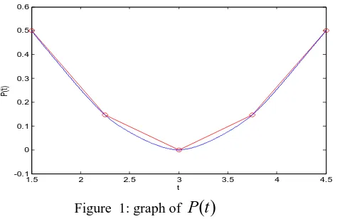
Example:Let ( ) = 2( / 6), [1.5, 4.5]
cos
f t t t with interpolating knots at
t
0=
1.5
,t
1=
2.25
,t
2=
3.00
,t
3=
3.75
,t
4=
4.5
,0.75
=
h
. let
=
0.99
, and letf
(
t
)
is the function being interpolated.Denote the corresponding C2-continuous interpolating function defined by(4)
in[1.5,4.5]
byp
(
t
)
since the interpolating data and parameter
satisfy the condition of theorem1
. asshown in figure
1
.1.5 2 2.5 3 3.5 4 4.5
-0.1 0 0.1 0.2 0.3 0.4 0.5 0.6
t
P
[image:5.612.203.442.399.553.2](t)
Figure 1: graph of
P
(
t
)
VI. APPROXIMATION PROPERTIES OF THE WEIGHTED RATIONAL QUADRATIC TRIGONOMETRIC INTERPOLATION
To estimate error of the weighted rational quadratic trigonometric interpolating function defined by (4), since the interpolation is
local,without loss of generality, we consider the error in the subinterval
[
t
i,
t
i1]
. When(
)
[
0,
]
2
n
t
t
C
t
f
and P(t) is the rationalquadratic trigonometric spline interpolating function of
f
(
t
)
in[
t
i,
t
i1]
. It is easy to see that this type of interpolation is exact for)
(
t
f
, the polynomial being interpolated,in which the degree is no more than1
. Consider the case when the knots are equallyspaced,namely,
n
t
t
h
h
ni
0
=
=
for alli
=
1,2,...,
n
,
using the Peano-Kernel Theorem in Schultz [13)
] gives the following]
,
[
,
d
]
)
[(
)
(
=
)
(
)
(
=
]
[
(2) 11
i
t i it
i t
t
t
t
t
R
f
t
P
t
f
f
where
2 1
1
<
<
)
(
<
<
)
(
<
<
)
(
=
]
)
[(
i i
i i
t
t
t
r
t
t
q
t
t
p
t
R
where
2 1
(1
)
( ) = (
)
{[
2 sin
(1
sin
)
(
)2 cos
(1
cos
)
2
2
2
2
2
(1
cos
) ](
)
2 cos
(1
cos
)} / (
cos
sin
),
2
2
2
2
2
i i
i i i
i i i
p
t
h
t
;
<
<
t
t
i
(10)2
1
(1
)
( ) = {[
2 sin
(1 sin
)
(
)2 cos
(1 cos
)
2
2
2
2
2
(1 cos
)
](
)
2 cos
(1 cos
)} / (
cos
sin
),
2
2
2
2
2
i i
i i i
i i i i
q
h
t
;
<
<
t
i1t
(11)
;
<
<
,
)
2
sin
2
cos
(
)
)(
2
cos
(1
2
cos
2
)
(1
=
)
(
1 22
i i
i i
i i
t
t
t
r
(12)
Then
1 2
2
1
|| [ ] || =||
( )
( ) ||
||
( ) || { |
( ) | d
| ( ) | d
| ( ) | d }
t t
t i i
ti t ti
R f
f t
P t
f
t
p
q
r
(13)
for
1
r
(
)
0
for all
[
t
i1,
t
i2]
, thus)
2
sin
2
cos
(
)
2
cos
(1
2
cos
)
(1
=
d
|
)
(
|
22
1
i i
i i
t
i t
h
r
(14)
for
q
(
)
, since]
)
2
cos
(1
)
2
cos
(1
2
cos
)2
2
(
)
2
sin
(1
2
sin
2
)
(1
)[
{(1
=
)
(
2
i ii i
h
t
q
0
)
2
sin
2
cos
)}/(
2
cos
(1
2
cos
2
i i
i
(15)
and
0
)
2
sin
2
cos
(
)
2
cos
(1
2
cos
2
=
)
(
1
i i
i i
h
t
q
(16)
It is easy to see that the root
* ofq
(
)
is]
)
2
cos
(1
)
2
cos
(1
2
cos
)2
2
(
)
2
sin
(1
2
sin
2
)
(1
[
)
2
cos
(1
2
cos
2
=
2 1
*
i i
i i
i i
h
t
Thus
*
1 1
2 1 *
| ( ) | d =
( )d
( )d =
[
]
ti ti
t t
q
q
q
h Q
)
2
)
(1
](
)
2
cos
(1
)
2
cos
(1
2
cos
)2
2
(
)
2
sin
(1
2
sin
2
)
(1
{[
=
22 2
2
1
h
z
Q
i ii
i
)
2
sin
2
cos
))}/(
(1
))(2
2
cos
(1
2
cos
2
(
i i
i
z
(17)
2
)
2
cos
(1
)
2
cos
(1
2
cos
)2
2
(
)
2
sin
(1
2
sin
2
)
(1
)
2
cos
(1
2
cos
2
=
i i
i i
i
z
(18)
2
)
2
cos
(1
)
2
cos
(1
2
cos
)2
2
(
)
2
sin
(1
2
sin
2
)
(1
{
[
=
)
(
i
i i i
i
h
t
p
0
)]
2
sin
2
cos
)}/(
2
cos
(1
2
cos
2
i i
i
(19)
and the root
* ofp
( )
in t t
[ , ]
i isN
M
h
t
i1
*=
where
)]
2
cos
(1
2
cos
2
)
2
sin
2
cos
1)(
[(
=
i
i i
h
M
(20)
)]
2
sin
2
cos
(
)
2
cos
(1
)
2
cos
(1
2
cos
)2
2
(
)
2
sin
(1
2
sin
2
)
(1
[
=
2
i i
i i
i i
N
(21)
so that
d
)
(
d
)
(
=
d
|
)
(
|
* *
p
p
p
t
i t t
i t
2 1 2
1 2
3
(1
)
[
2sin
(1 sin
) (
)2 cos
(1 cos
) (1 cos
) ](
)
2 cos
(1 cos
)
2
2
2
2
2
2
2
2
=
{
(
cos
sin
)
2
2
2
cos
(1 cos
)
2
2 }
(
cos
sin
)
2
2
i i i i
i i
i i
i
i i
h
t
h z
z
z
2 2
=
h
Q
where
]
)
)
((1
2
[
=
22
1
N
M
z
]
2
)
(1
2
1
[
=
2 2
2
N
M
z
)]
)
[(2(1
=
3
2 2
|| [ ] || =|| ( )
R f
f t
P t
( ) ||
h
||
f
( ) || ( ,
t
w
i,
i)
where
]
)
2
sin
2
cos
(
)
2
cos
(1
2
cos
)
(1
[
=
)
,
,
(
Q
1Q
2w
i i
i i
i
(22)
where
w
(
,
i,
i)
is a constant depending upon
,
i,
i.ACKNOWLEDGMENT
We are thankful to Prof. Xuli Han (Deptt. of Applied Mathematics and Applied Software, Central South University, Changsha, PR China) for his valuable suggestions.
REFERENCES
[1] Q. Duan, L. Wang and E. H. Twizell, “ A new weighted rational cubic interpolation and its approximation”, Appl. Math. Comput., 2005, 168, pp.990–1003. [2] M. Dube , R. Sharma , “Quadratic NUAT B-spline curves with multiple shape parameters”, International Journal of Machine Intelligence, 2011,3, pp.18–24. [3] M. Dube, S. Sanyal, “Shape preserving G2 rational cubic trigonometric spline”, Journal of the Indian Math. Soc., 2011, 78, pp.35–43.
[4] J. A. Gregory, “Shape preserving spline interpolation”, Comput. Aided Des., 1986, 18, pp.53–57.
[5] Xi. An Han., Ma. Yi. Chen, and Xi. Li Huang, “The cubic trigonometric Bézier curve with two shape parameters”, Applied Mathematics Letters, 2009, 22, pp.226-231.
[6] Xuli. Han, “Quadratic trigonometric polynomial curves with a shape parameter”, Computer Aided Geometric Design, 2002, 19(7), pp.503–512. [7] S. S. Rana, M. Dube, S. Sanyal “A GC 2 cubic trigonometric B-spline”, Investigation in Mathematical Sciences, 2011, 1, pp.25–31.
[8] M. Sarfraz, “Convexity preserving piecewise rational interpolation for planer curves”, Bulletin of Korean Mathematical Society, 1992,29, pp.193–200. [9] I. J. Schoenberg, “On trigonometric spline interpolation”, J.Math. Mech., 1964, 13, pp.795–825.
[10] M. H. Schultz, “Spline Analysis”,Prentice-Hall:Englewood Cliffs, New Jersey, 1973. AUTHORS
First Author – Mridula Dube, Ph. D., Professor, Department of Mathematics and Computer Science, R. D. University, Jabalpur, India
Second Author (Correspondence Author) – Preeti Tiwari, M. Sc., Astt. Professor, Department of Mathematics, G.G.I.T.S., Jabalpur, India.
Email address – preetitiwari1976@gmail.com Alternate email address– jaidev.tiwari@gmail.com Contact number. +919425860950