Volume 2010, Article ID 137428,9pages doi:10.1155/2010/137428
Research Article
A Lot-Size Model for Deteriorating
Items under Conditions of a One-Time
Only Extended Credit Period
Nita H. Shah
Department of Mathematics, Gujarat University, Gujarat, Ahmedabad 380 009, India
Correspondence should be addressed to Nita H. Shah,[email protected]
Received 16 July 2009; Accepted 20 January 2010
Academic Editor: Dalibor Froncek
Copyrightq2010 Nita H. Shah. This is an open access article distributed under the Creative Commons Attribution License, which permits unrestricted use, distribution, and reproduction in any medium, provided the original work is properly cited.
Now-a-days, the offer of credit period to the customer for settling the account for the units purchased by the supplier is considered to be the most beneficial policy. In this article, an attempt is made to formulate the mathematical model for a customer to determine optimal special cycle time when the supplier offers the special extended credit period for one time only during a special period. A decision policy for a retailer is developed to find optimal special cycle time. The theoretical results and effects of various parameters are studied by appropriate dataset.
1. Introduction
The most prevailing business strategy is adopted by the supplier to offer credit period of
say30 days to settle the account of the retailer. This strategy attracts new customers who consider it to be a type of discount strategy. The interest is not charged if the account is settled within the permissible credit period. However, if the payment is delayed beyond this period, the interest is charged for unsettled account. The retailer can earn the interest by putting generated revenue in an interest-bearing account. Thus, credit period reduces the amount of capital invested in stock, and thereby, reduces retailer’s holding cost of stock. When units in inventory are subject to deterioration, the cost of deterioration incurred by the retailer contributes to the total cost of an inventory system.
Goyal1developed an economic order quantityEOQmodel under conditions of permissible delay in payments. Shah2and Aggarwal and Jaggi3extended Goyal’s model for deteriorating items. Jamal et al.4generalized the model to allow for shortages. Teng5
Sarker et al.12, Shah13, Shah et al.14, Teng et al.15, Ouyang et al.16, Shah17, and many more.
The abovementioned developments assumed that a supplier provides his customer a credit periodsayM for settling the account during the normal period. Soni and Shah18
derived mathematical model under the assumption that the supplier offers one more credit periodsayN N > Mto the retailer for settling the account of the purchased goods.
In this paper, an attempt is made to extend the credit period only once during a specified period as a special marketing strategy to motivate the retailer to order larger than usual order quantities. The assumption of Teng 5 that the selling price is higher than the unit purchase cost is considered. The units in inventory are subject to constant rate of deterioration. The necessary and sufficient conditions for the optimal solutions are derived. The algorithm is constructed to find optimal special cycle time. The derived analytical results are illustrated with numerical examples.
2. Assumptions and Notations
2.1. Assumptions
The proposed mathematical model is derived with the following assumptions.
iThe annual demand for the product is deterministic and constant over time.
iiLead-time is zero. Shortages are not allowed.
iiiThe replenishment rate is infinite.
ivDuring the credit period, the generated revenue is deposited in an interest-bearing account at the rate ofIe/ $/unit/annum. At the end of the credit period, the retailer pays offfor all the sold units, keeps the profit, and pays for the interest charges on the items in the stock at the rate ofIc/$/unit/annum. In general,Ic > Ie.
vThe supplier offers a credit period, M for settling accounts during the normal period. However, during festival seasons, the supplier offers extended credit period ofNN > Mto settle the accounts during a given specified period. The customer has a chance to use this offer only once.
viThe units in inventory deteriorate at a constant ratesayθ0 ≤θ <1. The value ofθis small compared to those of other model parameters. The deteriorated units can neither be repaired nor replaced during a cycle time. The sensitivity analysis in Examples5.1and5.2is carried out by takingθ0.10.
2.2. Notations
The following notations will be used in building mathematical model.
iR: the annual demand.
iih: the inventory holding cost/unit/year excluding interest charges.
iiiIc: the interest charges/$ invested in stock/annum.
ivIe: the interest earned/$ in a year.
vP: the unit selling price of the item/unit.
viiA: the ordering cost/order.
viiiM: the usual credit period in settling the account.
ixN: the extended credit period in settling the account.
xT0: the regular cycle time when the credit period isM.
xiTs: the special cycle time when the extended credit ofN-time units is offered. xiiNT0: the minimum total annual cost during the periodT0.
xiiiKiTs: the total variable cost during the special cycle timeTsfor casei.
3. Mathematical Model
Following Goyal1and Shah2, we will derive mathematical models for the following two cases.
Case 1. LetTs≥N, that is, special cycle time is greater than or equal to extended credit period.
Under the assumption that the customer can make the use of extended credit offered by the supplier once, the total variable cost during the given specified period is given by
K1Ts A h CθR
θ2
eθTs−θT
s−1
CIcR
θ2
eθTs−N−θT
s−N−1
−P IeRN2
2 .
3.1
The total cost during cycle time under normal condition is given by TsNT0.
Therefore, the net cost of the system as a result of changing the payment scenario during the given specified time is given byZ1Ts K1Ts−TsNT0. To obtain minimum value of
Z1Ts, the necessary condition isdZ1Ts/dTs0, that is,
h CθR θ
eθTs−1
CIcR
θ
eθTs−N−1
−NT0 0, 3.2
and sufficient condition is
d2Z 1Ts
dT2
s
h Cθ CIce−θNReθTs >0. 3.3
We need to solve3.2forTs Ts1 by suitable numerical method. Assumingθ to be
very small, we take series approximation of exponential up toθneglectingθ2 and higher
powers. We get
h CIcθT2
s
2 {h Cθ CIc1−θN}Ts−CIcN
CIcθN2
2 −
NT0
which gives
TsTs1×
−{h Cθ CIc1−θN}
h CIcθ
{h Cθ CIc1−θN} −2h CIcθ−CIcN CIcθN2/2−NT
0/R
h CIcθ ,
3.5
To ensure thatTs1> N, we substitute3.5into inequalityTs1> Nand obtain that
NT0>
2h2 2CIch 2C2Icθ CIchθN h2θN 2ChθNR
2h CIc . 3.6
Case 2Ts< N. Following Shah2, the total variable cost during the given specified period
is
K2Ts A h CθR
θ2
eθTs−θT
s−1
P IeRTs
N−Ts
2
. 3.7
Arguing as above, the net cost incurred during the given specified period isZ2Ts K2Ts−
TsNT0. Under series approximation,Tsis given by
Ts
−h Cθ P Ie h Cθ P Ie2 2hθP IeN NT0/R
hθ , 3.8
and sufficient condition is
d2Z 2Ts
dT2
s
h CθReθTs P IeR >0. 3.9
Substituting3.8into inequalityTs< N, we get
NT0< RN{Nθh Cθ 2h Cθ−P Ie} 2P IeN
2 . 3.10
Postulate 1.
1If3.6holds, then the optimal cycle timeTs1for special credit period is given by
3.5.
2If3.10holds, then the optimal cycle timeTs2for special credit period is given by
3.8.
3If equality holds in3.6or3.10, then the optimal cycle time isNfor special credit period.
Proof. It follows from above discussions.
Using results of Shah2and above theorem, we have the following postulate.
Postulate 2. Let
Δ1 Rh Cθ P IeM2,
Δ2Rh CθN,
3.11
T01
2A M2RCIc−P Ie
h Cθ CIcR , 3.12
T02
2A
h Cθ P IeR. 3.13
1If 2A >Δ1and
iNT01>Δ2,then optimal cycle time isTs1for extended credit period.
iiNT01<Δ2,then optimal cycle time isTs2for extended credit period.
iiiNT01 Δ2,then optimal cycle time isN,the extended credit period.
2If 2A Δ1and
iNM>Δ2,then optimal cycle time isTs1for extended credit period.
iiNM<Δ2,then optimal cycle time isTs2for extended credit period.
iiiNM Δ2,then optimal cycle time isN,the extended credit period.
3If 2A <Δ1and
iNT02>Δ2then optimal cycle time isTs1for extended credit period.
iiNT02<Δ2then optimal cycle time isTs2for extended credit period.
iiiNT02 Δ2then optimal cycle time isN; the extended credit period.
Using Shah2, the minimum annual cost is
NT01 A
T01
h CθR θ2T
01
eθT01 −θT
01−1
CIcR
θ2T 01
eθT01−M−θT
01−M−1
−P IeRM2
2T01 ,
3.14
NT02 A
T02
h CθR θ2T02
eθT02 −θT
02−1
−P IeR
M−T02
2
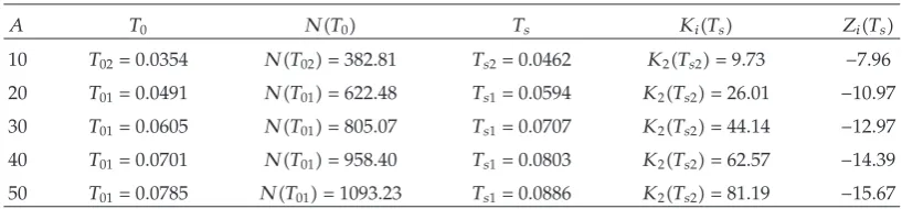
Table 1: Optimal solution for different ordering costs.
A T0 NT0 Ts KiTs ZiTs
10 T020.0354 NT02 382.81 Ts20.0462 K2Ts2 9.73 −7.96
20 T010.0491 NT01 622.48 Ts10.0594 K2Ts2 26.01 −10.97
30 T010.0605 NT01 805.07 Ts10.0707 K2Ts2 44.14 −12.97
40 T010.0701 NT01 958.40 Ts10.0803 K2Ts2 62.57 −14.39
50 T010.0785 NT01 1093.23 Ts10.0886 K2Ts2 81.19 −15.67
4. Algorithms
Step 1. If 2A >Δ1,then go to Algorithm A.
Step 2. If 2A Δ1,then go to Algorithm B.
Step 3. If 2A <Δ1,then go to Algorithm C.
Algorithm A. The steps are as follows.
A.0ComputeT01using3.12andNT01using3.14.
A.1IfNT01>Δ2,then optimal solution isTs1, K1Ts1.
A.2IfNT01<Δ2,then optimal solution isTs2, K1Ts2.
A.3IfNT01 Δ2,then optimal solution isN, K1N K2N.
Algorithm B. The steps are as follows.
B.0SetT Mand calculate
NM A
M
h CθR θ2M
eθM−θM−1−P IeRM
2 . 4.1
B.1IfNM>Δ2,then optimal solution isTs1, K1Ts1.
B.2IfNM<Δ2,then optimal solution isTs2, K1Ts2.
B.3IfNM Δ2,then optimal solution isN, K1N K2N.
Algorithm C. The steps are as follows.
C.0ComputeT02using3.13andNT02using3.15.
C.1IfNT02>Δ2,then optimal solution isTs1, K1Ts1.
C.2IfNT02<Δ2,then optimal solution isTs2, K1Ts2.
Table 2: Optimal solution for extended credit period.
N Δ2 Ts KiTs ZiTs
30/365 493.15 Ts20.0963 K2Ts2 49.97 −8.53
45/365 739.73 Ts10.1065 K2Ts2 46.17 −18.53
60/365 986.30 Ts10.1167 K2Ts2 40.84 −30.06
75/365 1232.88 Ts10.1268 K2Ts2 33.96 −43.07
Table 3: Effect of deterioration of units on optimal solution.
Θ Δ1 Δ2 T01 NT01 Ts1 KiTs1 ZiTs1
0.10 14.19 493.15 0.0861 607.50 0.0963 49.97 −8.53
0.15 15.88 575.34 0.0812 649.70 0.0902 50.55 −8.05
0.20 17.56 657.53 0.0770 689.66 0.0851 51.04 −7.65
0.25 19.25 739.73 0.0734 747.70 0.0809 51.47 −7.40
5. Numerical Examples
Example 5.1. Consider the data
R, h, Ic, Ie, C, P, M, N, θ
2000,4,0.10,0.08,20,30, 15
365, 30 365,0.10
5.1
in appropriate units. ThenΔ1 28.37 andΔ2 986.30. Using The Algorithms A–C., let us
tabulate computational results forA10, 20, 30, 40, and 50 inTable 1.
It is observed that increase in ordering cost increases T0,NT0, Ts,and KiTs but
decreases the net costZiTs.
Example 5.2. Consider the data
R, h, Ic, Ie, C, P, A, M, θ
1000,4,0.10,0.08,20,30,30, 15
365,0.10
5.2
in appropriate units. Then 2A 60 > Δ1 14.19. Using Algorithm A, we getT0 T01
0.0861 andNT01 607.50. Let us study effect of extended credit periodNon the decision
variables inTable 2.
It is observed that increase in extended credit period increasesΔ2 and special cycle
time but decreases in the total annual cost of an inventory system and net cost.
Example 5.3. Consider the data
R, h, Ic, Ie, C, P, A, M, N
1000,4,0.10,0.08,20,30,30, 15
365, 30 365
5.3
[image:7.600.96.505.227.305.2]Increase in deterioration of units in inventory system lowers normal cycle time, special cycle time, net cost, and increase in total annual cost of an inventory system and special credit period policy.
6. Conclusions
In this article, we extended classical EOQ model for a retailer when units in inventory are subject to deterioration at a constant rate and supplier offers only one-time extended credit period to settle retailer’s account. Under series approximation of exponential term, a closed-form solution of optimal cycle time is obtained. The algorithms are provided for determining optimal policy.
Acknowledgment
The author is thankful to reviewer for his suggestions to improve the research article.
References
1 S. K. Goyal, “Economic ordering quantity under conditions of permissible delay in payments,” Journal of the Operational Research Society, vol. 36, pp. 335–338, 1985.
2 N. H. Shah, “A lot—size model for exponentially decaying inventory when delay in payments is permissible,” Cahiers du Centre D’ Etudes de Recherche Operationnell, vol. 35, pp. 1–9, 1993.
3 S. P. Aggarwal and C. K. Jaggi, “Ordering policies of deteriorating items under permissible delay in payments,” Journal of the Operational Research Society, vol. 46, pp. 658–662, 1995.
4 A. M. M. Jamal, B. R. Sarker, and S. Wang, “An ordering policy for deteriorating items with allowable shortage and permissible delay in payment,” Journal of the Operational Research Society, vol. 48, pp. 826–833, 1997.
5 J.-T. Teng, “On the economic order quantity under conditions of permissible delay in payments,” Journal of the Operational Research Society, vol. 53, pp. 915–918, 2002.
6 N. H. Shah, “A probabilistic order level system when delay in payments is permissible,” Journal of the Korean Operations Research and Management Science, vol. 18, no. 2, pp. 175–183, 1993.
7 N. H. Shah, “Probabilistic time scheduling model for exponentially decaying inventory when delay in payments is permissible,” International Journal of Production Economics, vol. 32, pp. 77–82, 1993.
8 H. Hwang and S. W. Shinn, “Retailer’s pricing and lot—sizing policy for exponentially deteriorating products under the condition of permissible delay in payments,” Computers and Operations Research, vol. 24, pp. 539–547, 1997.
9 A. M. M. Jamal, B. R. Sarker, and S. Wang, “Optimal payment time for a retailer under permitted delay of payments by the wholesaler,” International Journal of Production Economics, vol. 66, pp. 59–66, 2000.
10 H. C. Liao, C. H. Tsai, and C. T. Su, “An inventory model with deteriorating items under inflation when a delay in payments is permissible,” International Journal of Production Economics, vol. 63, pp. 207–214, 2000.
11 C.-T. Chang, L.-Y. Ouyang, and J.-T. Teng, “An EOQ model for deteriorating items under supplier credits linked to ordering quantity,” Applied Mathematical Modeling, vol. 27, pp. 983–996, 2003.
12 B. R. Sarker, A. M. M. Jamal, and S. Wang, “Optimal payment time under permissible delay for production with deterioration,” Production Planning & Control, vol. 11, pp. 380–390, 2001.
13 N. H. Shah, “Probabilistic order level system when items in inventory deteriorate and delay in payments is permissible,” Asia—Pacific Journal of Operational Research, vol. 21, no. 3, pp. 319–331, 2004.
14 B. J. Shah, N. H. Shah, and Y. K. Shah, “An order—level lot-size model with stock dependent demand for time dependent deterioration under permissible delay in payments,” Far East Journal of Theoretical Statistics, vol. 12, no. 2, pp. 201–220, 2004.
16 L.-Y. Ouyang, J.-T. Teng, K.-W. Chuang, and B.-R. Chuang, “Optimal inventory policy with non instantaneous receipt under trade credit,” International Journal of Production Economics, vol. 98, no. 3, pp. 290–300, 2005.
17 N. H. Shah, “Inventory model for deteriorating items and time value of money for a finite time horizon under the permissible delay in payments,” International Journal of Systems Science, vol. 37, no. 1, pp. 9–15, 2006.