Volume 2011, Article ID 862813,19pages doi:10.1155/2011/862813
Research Article
On the Sodium Concentration Diffusion with
Three-Dimensional Extracellular Stimulation
Luisa Consiglieri and Ana Rute Domingos
Departamento de Matem´atica e CMAF, Faculdade de Ciˆencias da Universidade de Lisboa, 1749-016 Lisboa, Portugal
Correspondence should be addressed to Luisa Consiglieri,[email protected]
Ana Rute Domingos,[email protected]
Received 3 December 2010; Revised 1 March 2011; Accepted 20 May 2011
Academic Editor: Brigitte Forster-Heinlein
Copyrightq2011 L. Consiglieri and A. R. Domingos. This is an open access article distributed
under the Creative Commons Attribution License, which permits unrestricted use, distribution, and reproduction in any medium, provided the original work is properly cited.
We deal with the transmembrane sodium diffusion in a nerve. We study a mathematical model of a
nerve fibre in response to an imposed extracellular stimulus. The presented model is constituted by a diffusion-drift vectorial equation in a bidomain, that is, two parabolic equations defined in each
of the intra- and extra-regions. This system of partial differential equations can be understood
as a reduced three-dimensional Poisson-Nernst-Planck model of the sodium concentration. The representation of the membrane includes a jump boundary condition describing the mechanisms involved in the excitation-contraction couple. Our first novelty comes from this general dynamical boundary condition. The second one is the three-dimensional behaviour of the extracellular stimulus. An analytical solution to the mathematical model is proposed depending on the morphology of the excitation.
1. Introduction
predictions, the well-known Hodgkin-HuxleyHH for shortmodel plays an essential role for the quantitative understanding of the biological phenomena 4. This work proposed that the action of potential in axon membranes can be analysed using cable theory. The authors proposed a system of four ordinary differential equations ODEs describing the current clamped experiments. Indeed, the previously unobserved dynamics in the HH model has a chaotic behaviour5. The field of computational neurophysiology has a long history containing extensive studies about the excitation of neural elements6,7. A constructive discussion on the appropriate modelling of neural structures and their stimulation and blocking activities, by electrodes relatively remote from the target nerve cell, is provided in 6. Rattay’s book 7 illustrates whether the classical results for propagating action potentials, say the HH model for nonmyelinated fibres and the Frankenhauser-Huxley model for myelinated fibres, and subsequent analytical and numerical models may embody the phenomena and fit the electrophysical experiments.The nerve cell or neuron is constituted by the soma the cellular body, the dendrite, and one axon that connects the previous two. Some neurons have axons with an insulating layer, discontinuous, the so-called myelin sheath. These are the myelinated fibres. Neurons with naked axons, that is axons without myelin covering, are the so-called unmyelinated fibres 8. Modified ODE systems 9–
14 have extended the standard HH model and have been analysed through phase space methods where equations are not explicitly solved. The control theory of the nonlinear systems exhibits chaotic behaviour of the version also known as the Fitzhugh-NagumoFN model that consists of a second-order ODE dealing with the variation in time of the gating quantities and reinterprets the model developed by Hodgkin-Huxley9. Fitzhugh in10
deals with a stable state and threshold phenomena as well as stable oscillations described by two variables of state, representing excitability and refractoriness, which are solutions of the so-called Bonhoeffer-van der Pol model. An extended FN system of ODE is numerically integrated in two different one-dimensional situations: free fibre and an externally stimulated clamped one11. A second-order differential equation of generalised FN type is solved by the least squares method, having as a solution the given single componentaction potential of the numerical solution12. Other variants of the HH model can be found in13, based on geometric singular perturbation theory. Dynamics of spike initiation in other simplifications of the HH model, namely, the Morris-Lecar model, is exploited with phase plane and bifurcation analysis14.
Recently, using the Green function’s method, analytic solutions for the cable equation response to the extracellular stimulus current have been found 15. This alternative interpretation of the situation is the first step to understand the behaviour of the potential solution.
Our concern is to understand the dynamics on the electrodiffusion of charged molecules in particular, Na ions. We refer to 16, 17 for the 3D Poisson-Nernst-Planck PNP model analysed by finite element methods. Using a dynamic lattice Monte Carlo model 18, a description of the electrochemical processes is provided for the ion transport. After the reduction of the PNP model to a system of first-order ODE, in 19 the construction of singular orbits and the application of geometric singular perturbation theory provide information over permanently charged ions flow through an ion channel.
interface itself. In 21, the convergence of an electrochemical model is shown for a mixture of charged particles in a solution subject to prescribed electric potentials at two electrodes into a unique steady-state boundary value problem. An alternative approach, modelling the transmembrane potential in electrocardiology 22, considers a bidomain with a dynamic boundary jump condition, which is closely related to ours.
The membrane dynamics used in this paper is based on the mathematical model started in the work 23. Our model is derived from the Maxwell equations with current density defined by the Fick-Ohm law. Then, a drift term is included by the electrical contribution, which does not happen in the diffusion formulations obtained by mass and momentum conservation laws.
Experimentally, an action potential is often generated by a rapid injection of current at a fixed point in the resting axon, which then spreads from the point of stimulation. However, the nerve cell is a three-dimensional structure. Even if a stimulus current pulse is arranged by the insertion of an electrode, a local current is developed. The membrane potential of the cell is not uniform at all points. The depolarisation spreading passively from an excited region of the membrane near the insertion region of the electrode to a neighbouring unexcited region occurs in three dimensions until uniformity is reached. This means that there is an interval of time where the flow has an angular dependence. The discrepancy between theory and experiments depends on the configuration of the experimental apparatus from which the propagated action potential was initiated and the strength of the current used to generate it
24. Indeed, the discrepancy between the theoretical predicted and reported speeds of the propagated action potential is a consequence of neglecting the radial variation that occurs over small distances by comparison with axonal length. In24, Fourier spectral methods are used to construct periodic solutions of the intracellular and extracellular potential for the Laplace equation.
The goal of the present study is to determine how the profile of the activation affects the time parameter and the 3D domain of action potential initiating and, consequently, the propagation. This nonlinear model highlights the fact that an action potential is not generated instantaneously when the membrane potential crosses some preordained threshold25. We refer to26 where the excitation response of an idealised infinite fibre is evaluated from the applied field of a unique point source electrode. Our main new contribution relies on the angular dependence of the concentration, since the stimulation can reliably propagate in a 3D form25. The description of the physiological phenomenon will be more realistic with 3D models. Moreover, we assume no azimuthal symmetry because it reflects the physical character of the biological phenomenon. In sum, we believe that these features can contribute to remove the actual discrepancy between the predicted and observed speed of the propagated action potential.
Several biological constants are used throughout the paper. We keep them abstract so that the presented solution can be applied on different biological contexts. We illustrate their values with some examplessquid, cat, etc..
2. Statement of the Problem
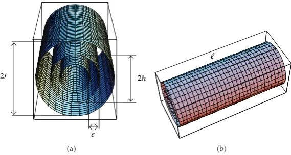
The axon is a thin cellular extension, that may be short or long, responsible for transporting the information electrical impulses from the soma to the dendrite1. The axon can be described as a cylinder of lengthand radiush, surrounded by a membraneΓmof negligible
thicknessthe cylinder surfaceand immersed in an extracellular medium
Ωe:x, y, z
∈R3: 0< x < , h2< y2z2 < r2, 2.1
for some 0 < h < r seeFigure 1. Let Ω ⊂ R3 be a neighbourhood of the membrane Γ
m
defined as
Ω:x, y, z∈R3: 0< x < ,h−2 < y2z2< r2, 2.2
for some 0< < h. ThusΩi: Ω\ΩeandΓm: Ω\Ωi∪Ωedenote the intracellular space
and the membrane surface, respectively. Define the external boundary
Γ: 0;×y, z∈R2:y2z2r2. 2.3
Let T > 0. The problem under study is defined by the system of parabolic equations for details see23
∂ci
∂t −D∇ 2c
i σi
εci0 in Ωi×0, T,
∂ce
∂t −D∇ 2c
e σe
ε ce0 in Ωe×0, T,
2.4
where D is the sodium diffusion coefficient D 0.267 ×10⁻⁹m2s−1, 27 and ε is the
sodium permittivity ε 6.4 ×10⁻¹⁰F m−1. The instant of timet is measured in seconds,
∂/∂t denotes the time derivative, and∇2 represents the Laplacian. Here, c
e and ci denote
the sodium concentration, respectively, inΩeand inΩi, measured in mol m−3. The electrical
conductivityσs, withs∈ {i, e}, is considered homogeneous and constant at each subdomain
extra- and intracellular domains, measured in S m−128:
σe
1
3 inΩe, σi 5
3 inΩi. 2.5
Other values for the diffusion coefficient and the electrical conductivity can be found in29. We assume the following boundary conditions:
∇ce·nΓ0 on Γ×0, T, 2.6
α∂
2h 2r
ε
a
ℓ
[image:5.600.157.442.96.248.2]b
Figure 1: Schematic representations of the axon and its extracellular mediumnot in scalein thex-axis
direction from the inputx 0to the outputx sitesthis figure was produced by the function
ParametricPlot3D of the software Mathematica 5.2 developed by Wolfram Research, and Microsoft Office
Power Point.
where nΓ and n denote the outward normal to Γ and Γm, respectively. The insulating
boundary condition in 2.6 represents the zero outflow. The interface condition in 2.7
governs the evolution of the discontinuity of the concentration, taking into account that the concentration jumpsc: ce−ci across the membrane satisfy a dynamical condition20.
Due to many conducting channels the lipid axon membrane exhibits a capacitive/conducting behaviour. It separates internal and external conducting solutions. Such a gap between two conductors forms a significant electrical capacitor. In living cells, the ions lost via ionic channels by diffusion are returned by ionic pumps in order to overcome the electrochemical gradient27. We can distinguish three main states of the channel: open, closed, and inactive. The opening of those channels requires several gating events. As in 20, 23, the gating functions are assumed positive real constants.
At the instantt 0, an external stimulusΦ, which can be electrical, mechanical, or chemical, is applied to depolarise the resting membrane. On the external region in the two-dimensional boundary{x0}the following condition holds:
∇ce·n
0, y, z,0 Φy, z, 2.8
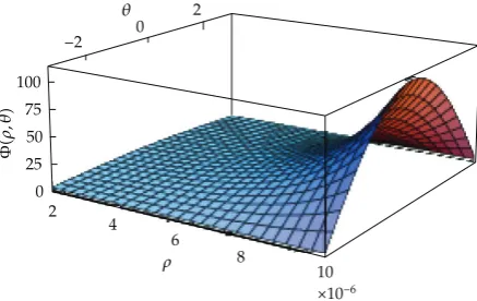
where n 1,0,0. The 1D propagation behaviour of an external stimulus has a peak in the axon initial segment induced by the realor simulatedsynaptic inputs30,31. Our firing pattern plotted inFigure 2corresponds to the 3D description. In the sequel, the 3D domain is considered defined in cylindrical coordinates, that is, thex-axis indicates the longitudinal distance along the length of the axon,ρ-axis the radial distance measured from the centre, andθ-axis the angular measure that performs the real three-dimensional feature of the axon behaviour. Then, the functionΦcan be given by
Φρ, θκ1ρ−1/2exp
τρκ2ρ1/2
cos
θ
−2 0 2 θ
0 25 50 75 100
Φ(
ρ,
θ
)
ρ 2
4 6
8
10
[image:6.600.190.409.98.236.2]×10−6
Figure 2: Adimensional plot of the mappingΦconsidered in2.9, forρ, θ∈h;r×−π;π. The plotted
surface illustrates the qualitative behaviour as function of the radiusρand the angleθ, at the input site
x0and the initial instant of timet0 this figure was produced by Mathematica 5.2, developed by
Wolfram Research.
withκ1, κ2, τ ∈ R, for everyρ, θ ∈h;r×−π;π seeFigure 2. The angular positionθ
0 corresponds to the closeness to the external source for the interval of time that current redistribution is not concludedsee7, page 154, e.g., for the monopolar electrode.
The initial condition is assumed constituted by an averaged condition:
Ωici·,0 Ci,
Ωece·,0 Ce, 2.10
with the values ofCiandCedepending on the physiological datae.g., in a cat motoneuron
Ci 15 mol m−3 andCe 150 mol m−3 cf.3, and for values at the various axons we refer
to32,33and references therein.
Finally, in order for the model to be accurate the Boltzmann principle must be satisfied. For this purpose, it will be sufficient for the validation of the effect of the concentration ratio through the membrane to be commensurable with the corresponding Nernst potentialNin the resting state, that is, at instancet0 and onΓm
ce
ci ρh,t0 N:exp
FzNaVd RTr
, 2.11
where Vd represents the depolarisation voltage, F is the Faraday constant F 9.649 ×
104C mol−1,3,Rdenotes the universal gas constantR8.314 Jmol·K−1, andT
rdenotes
the reference absolute temperature, in Kelvin.
3. Analytical Solution
In this section we present an analytical solution for2.4, forsi, e. For the sake of simplicity in notations, we will omit the indexswhen we look only at the generic equation. When we also take into account the boundary and the initial conditions, we will denote with an index
In cylindrical coordinates, both equations in2.4read as follows:
∂c ∂t −D
∂2c ∂x2
∂2c ∂ρ2 1 ρ ∂c ∂ρ 1 ρ2 ∂2c ∂θ2
σ
εc0, 3.1
with x, ρ, θ, t ∈0, ×h −, r×− π, π×0, T. Indeed, the above system of parabolic equations is considered together with the set of additional restraints 2.6–2.11. The validation of the initial and the boundary conditions specifies the choice of the several constants involved in the characterisation of the solutions, namely,ξ,δ0,i,δ1,i,δ2,i, ι, andη
seeSection 4. Thus, we get a solutionseeSection 3.1, for details:
ce
x, ρ, θ, t 1 ξ
κ1ρ−1/2exp
τρκ2ρ1/2
exp
ξx
ξ2D−σe ε t
cos
θ
2 , 3.2
withξgiven by3.25, and
ci
x, ρ, θ, t:
δ1,iρ−1/2exp
ξx ξιρ
ξ2D−σe ε t
δ2,iρ−1/2exp
ηιρδ0,iρ1/2
exp
ηx
η2D−σi
ε t cos
θ
2 ,
3.3
whereδ0,i,δ1,i,δ2,i, ι, andηare correlated such that3.31–3.38hold.
3.1. A Formal Derivation
Here we show an analytical solution for2.4. First we study the differential equation3.1; then we find an explicit solution for both the extra- and intracellular concentrations. Inspired by the Fourier method of separation of variables, a useful method for finding a solution of a partial differential equation with several variables, we look for a solution of the form
cx, ρ, θ, tYx, ρ, tZθ. 3.4
Consequently, from substituting this in3.1we obtain
−1
D ∂tY
Y ∂xxY
Y ∂ρρY
Y
1
ρ ∂ρY
Y 1 ρ2 Z Z − σ
Dε0, 3.5
where∂κY:∂Y/∂κand∂κκ∂2Y/∂κ2, forκ∈ {t, x, ρ}. Then there existsλ∈Rsuch that
Zθ λZθ,
λ
1
D
∂tY
Y
x, ρ, tσ ε −
∂xxY
Y
x, ρ, t−∂ρρY Y
x, ρ, t− 1 ρ
∂ρY
Y
x, ρ, t
ρ2.
Remark 3.1. The second-order ordinary differential equation for Z has the following solutions. Ifλ <0, then there exist real constantsd1,d2such that
Zθ d1cos
|λ|θ d2sin
|λ|θ ; 3.7
ifλ0, then there exist real constantsd1,d2such thatZθ d1θd2;
ifλ >0, then there exist real constantsd1,d2such that
Zθ d1exp
λθd2exp
−λθ. 3.8
We observe that the validation of the phenomenal data yields the choice of λ < 0 and bounded.
ByRemark 3.1,λis negative. Thus, the second-order ordinary differential equation for
Z has the solution given by3.7, where d1, d2 are real constants. Since we are interested in a nonnegative valued solution for 2.4, we assume thatY andZ are both nonnegative functions. Then, from3.7we get
Zθ dcos
|λ|θ , 3.9
withdnonnegative real constant. We will now analyse the second equation from3.6, that is,
ρ2
∂xxY ∂ρρY−
1
D∂tY− σ DεY
ρ∂ρYλY 0. 3.10
Inspired by the theory for the confluent hypergeometric equations see the appendix, we look for a function of the form
Yx, ρ, tρ−
√
|λ|ux, ρ, tρ√|λ|vx, t 3.11
that satisfies3.10, where
ux, ρ, t
∞
j0
fj
xρpDtjexpaxbρqDt, 3.12
anda,b,p, andqare real constants to be chosen later. Solving3.10forρ√|λ|v, we get
∂xxv− 1
D∂tv− σ
Thus, we choosesee34
vx, t v0exp
ξx
ξ2D−σ ε t
, 3.14
withξ∈R, andv0>0 in order to get positive solutions. Solving3.10forρ−√|λ|u, we obtain
∞
j0
2j1j2fj22ab−pj1fj1
a2b2−q− σ εD fj
·xρpDtj0.
3.15
3.1.1. Exterior Case
For simplicity, we will keep the unknown constants λ,d, fj,p, a, b,q, v0, and ξ without
the extracellular subscripts. In order to find the extracellular concentrationce, we use the
Neumann boundary condition2.6in cylindrical coordinates. Thus, from3.11–3.14we get
∞
j0
j1fj1
b−
|λ|
r
fj
xrpDtj
−|λ|r2√|λ|−1v0exp
ξ−ax−br
ξ2−q− σe εD Dt
.
3.16
Applying the Taylor formula inx−x0, withx0 −rpDt, and denotingUj j!fj, we
have
Uj1
b−
|λ|
r
Uj−
|λ|r2√|λ|−1v
0ξ−aj
×exp
a−ξ−br
a−ξpξ2−q− σe εD Dt
.
3.17
Since there is no dependence in time, we get
ξ−apqξ2− σe
εD. 3.18
DenotingM:b−|λ|/randN:−|λ|r2√|λ|−1v
0expa−ξ−br, it follows that
Uj1−MUjNξ−aj,
Uj2 M2UjN−Mξ−aξ−aj.
From3.15it follows that
2Uj22ab−pUj1
a2b2−q− σe
εD Uj0. 3.20
Thus, introducing3.19into3.20and using3.18, after some calculations we obtainUj
ξ−ajf0, with
f0
|λ|r2√|λ|−2v
0expa−ξ−br
2ξr2|λ| −pr
a−b22a−b|λ|/r2|λ|/r2pbξ−a−|λ|/r−ξ2. 3.21
Thus,
ue
x, ρ, tf0exp
ξx ξ−abρ
ξ2− σe εD Dt
, 3.22
and consequently
Ye
x, ρ, tf0ρ−
√
|λ|expξ−abρv0ρ√|λ|·exp
ξx
ξ2D−σe ε t
. 3.23
Notice that it still remains to findλ,d,a,b,v0, andξ. Using2.8,3.9, and3.23, we
obtain|λ|1/2hence,λ−1/4,dκ1/f0ξ,b−aτ−ξ, andv0f0κ2/κ1, concluding
that
ce
x, ρ, θ, t 1 ξ
κ1ρ−1/2expτρκ2ρ1/2exp
ξx
ξ2D−σe ε t
cosθ
2. 3.24
Finally, the initial condition2.10yields
expξ−1
ξ
κ1
r
h
ρ1/2expτρdρ2
5κ2
r5/2−h5/2 Ce
4 . 3.25
This means thatξis well defined.
3.1.2. Interior Case
We are interested in finding the intracellular concentration ci using the forms 3.12 and
3.14:
ci
x, ρ, θ, t
dρ−1/2ux, ρ, tδ0,iρ1/2exp
ηx
η2D− σi
ε t cos θ
2, 3.26
withδ0,idv0κ2/ξandλ−1/4. Here, we consider new unknown constantsd,fj,p,a,b,
First, notice that 3.15 is verified under these new unknown constants, and again
3.15implies3.20withσereplaced byσi, that is,
2Uj2
2ab−pUj1
a2b2−q− σi
εD Uj0. 3.27
Next, we verify2.7. Introducing3.24and3.26in2.7, we obtain
∞
j0
dαpDfj1j1αqDβfj
xhpDtj
−δ0,ihexp
−bhη−ax
η2D−σi
ε −qD t
α
η2D−σi ε β
exp
−bh ξ−axξ2D−σe/ε−qD
t ξ × κ1 α
ξ2D− σe
ε βD
1 2−hτ
expτh
κ2h
α
ξ2D− σe
ε β− D
2
.
3.28
Arguing as in the exterior caseseeSection 3.1.1, we can apply the Taylor formula inx−x0
withx0−hpDtresulting in for each time level,
Uj1−MUjNξ−ajP
η−aj,
Uj2M2UjN−Mξ−aξ−ajP
−Mη−aη−aj,
3.29
whereM:q/pβ/αpDand
Pt:− δ0,ih
dαpDexp
a−η−bha−ηpη2− σi
εD −q Dt
×
α
η2D−σi
ε β ,
Nt: 1
dαpDξexp
a−ξ−bh
a−ξpξ2− σe
εD−q Dt
× κ1 α
ξ2D−σe
ε βD
1 2 −hτ
expτh
κ2h
α
ξ2D−σe ε β−
D
2
.
Introducing3.29into3.27, we conclude thatdUjj!dfj ξ−ajδ1,i η−ajδ2,i,
where
δ1,i
d 2N
M−ξ−bp/2
2M2−M2ab−pa2b2−q−σi/εD , 3.31
δ2,i
d 2P
M−η−bp/2
2M2−M2ab−pa2b2−q−σ
i/εD
. 3.32
This implies the existence of the solution 3.3 if there is time independence in3.31and
3.32. This time independence can be given into3.30implying
η−apqη2− σi
εD, 3.33
ξ−apqξ2− σe
εD. 3.34
These mean that the constantspandqare well defined, andPt≡PandNt≡Nfor allt. Notice that the constantsδ1,i, andδ2,iare well defined observing that the constantsa,
b,δ0,iandηwill be known. For the sake of simplicity, if we takeιb−a, then3.26leads us
to3.3. Thus, condition2.10reads
Ci
4
expξ−1
ξ δ1,i
h
h−
ρ1/2expξιρdρexp
η−1
η
×
δ2,i
h
h−
ρ1/2expηιρdρ2δ0,i
5
h5/2−h−5/2.
3.35
This yields the choice forη. Finally, from2.11it follows that
1
ξ
k1
√
hexpτh k2
h expξx
N
δ1,i √
hexpξx ξιh δ2,i √
hexp
ηxηιhδ0,i
hexpηx ,
3.36
for allx∈0, . Hence, the algebraic system forιandδ0,iis
1
ξ
k1
√
hexpτh k2
h N√δ1,i
hexpξιh, 3.37
δ0,i−
δ2,i
h exp
ηιh, 3.38
4. Results and Discussion
Our continuum model 2.4–2.11 is developed to identify and analyse the diffusion phenomena, focusing on the average density distribution of species of charged particles and their description through unified partial differential equationsPDEs. We showed that these PDEs admit the existence of explicit solutions3.2and3.3for the intra- and extracellular sodium concentrations with well-determined constants, namely,
iκ1,κ2, andτcome from the profile of the extracellular stimulation2.9,
iiξ is given by 3.25, which is calculated from the initial condition2.10 for the intracellular sodium concentration,
iiiη is given by3.35, which is calculated from the initial condition2.10for the extracellular sodium concentration,
ivι and δ0,i are determined in 3.37 and 3.38, which come from the Boltzmann
principle2.11,
vδ1,i and δ2,i are determined in 3.31 and 3.32, which come from the jump
condition2.7.
This result relates to the underlying mechanisms of electrodiffusion in sodium ions. However, we emphasise that it can be applied to any charged particles.
The axon membrane acts as an interface between the intra- and extracellular concentrations of the Na ions where a dynamical jump condition is taken into account
see 2.7. This avoids studying the ionic diffusion across the membrane. Indeed, the membrane is regarded such that the sodium concentration defined in the whole domain may suffer a finite jump when the membrane surface is crossed. The limit values of the sodium concentration may not, therefore, be the same when the membrane is approached from either the exterior or the interior. The concentration difference between the outside and inside of the membrane in2.7transports ions against their concentration gradientsfrom regions of high concentration to regions of low concentration. Therefore, this jump interface condition includes the continuous process of autotransformation of the membrane due to the movement of the proteins that transport ions. The first time derivative produces irreversible motion due to the exponential time-dependent factor. In order to determine the validity of the presence ofαandβin2.7, we pay attention to the HH model, as most of the models in electrophysiology are either its variants or its simplifications. The sodium conductanceGNa, measured in S m−2, is regulated by voltage-dependent activation and inactivation variables
usually called gating variables. The sodium conductance of the squid axon membrane is a product of three terms: a scale factor termgNa, a turning-on processm3, and an inactivating processh, where mandhdenote the activation and the inactivation of the sodium current, respectively3,4,7:
Their dynamics are described by the ODE system:
dm dt
0.125−V
exp25−V/10−11−m− 4 expV/18m,
dh dt
0.07
expV/201−h−
1
exp30−V/10 1h,
4.2
where V Vm−VNa, withVm and VNa representing the membrane potential and sodium
equilibrium potential, in mV. This formulation expresses that the sodium conductance activation and inactivation are decoupled variables. A revised version of the HH model based on the molecular reaction sequence to account for both sodium and potassium conductance transients Goldman-Hodgkin-Katz equation was introduced by Clay 35. Other kinetic cycles were proposed in36and references therein. Clearly, all these coincide with the HH model when one species is taken into account. Therefore, if the thickness of the membrane has a positive Lebesgue measure, the sodium conductance system can be modelled by expressing the kinetic model output as
I Cm
∂V
∂t Vm−VNaGNa, 4.3
with Cm denoting the membrane capacitance F m−2. Since4.2 has usually been solved
under steady-state gating functions, which means thatV ≡Vx, then, passing to the limit as the thickness tends to zero, the steady-state conduction gives the characterisation
β∼σm
membrane conductivity, 4.4
considering the Poisson equation to compute the electric field from the charge present into the system
−∇ ·ε∇V Fzc. 4.5
Using a time-dependent argument,αis correlated with the membrane permittivity. We refer to37, a study of the electrical properties of the cell surface, known as the membrane.
Also, our model fits the PNP model. Considering only one species, this electrodiffusion model is constituted by the Nernst-Planck equation to compute the ionic flux in an electrochemical gradient, in our notations,
∂c
∂t ∇ ·D
∇c Fz
kBT
c∇V 0, 4.6
Finally, we discuss how powerful is the technique executed here for the finding of explicit solutions to similar models. For instance, if we take the model from38, withciand
cegiven by3.26and3.24, respectively,
∂ci
∂t αce−βci, 4.7
then equality3.28reads
∞
j0
dpDfj1j1qDβtfj
xhpDtj
−αtδ0,ihexp
−bhη−ax
η2D−σi
ε −qD t
exp
−bh ξ−axξ2D−σ
e/ε−qD
t ξ
×
κ1
αt D
1 2 −hτ
expτh κ2h
αt− D
2
,
4.8
observing thatα≡αtandβ≡βt. Therefore, it follows thatMt:q/pβt/pD,
Pt:−αtδ0,ih
dpD exp
a−η−bha−ηpη2− σi
εD −q Dt
,
Nt: 1
dpDξexp
a−ξ−bh
a−ξpξ2− σe
εD −q Dt
×
κ1
αt D
1 2 −hτ
expτh κ2h
αt−D
2
.
4.9
As in Section 3.1, expressions 3.31 and 3.32, with these new expressions, imply the existence of the solution 3.3if there is independence in time. Thus, new relations can be obtained between the unknown constants of the executed technique and the physiological data, observing that the gating functions have exponential forms. Notice that the extracellular concentration keeps its definition, and this new jump condition4.7infers new constants into the definition for the intracellular concentration.
The mobility of sodium channels, the mechanisms by which they are distributed over neurons, and the maintenance of this distribution are important issues for the physiology of excitable cells. Recent progress in determining 3D structures of biomolecules such as ion channels greatly facilitates the diffusion continuum description; see, for instance,39. The theory behind electrodynamics turns into the electrobiology by studying the diffusing channels which are simply reflected by the boundary.
5. Conclusions
angularly distributed nature plays a crucial role in determining the action potential initiation. The sinusoidal shape over the angular structure is not documented in the literature since the experimental studies are devoted to the radial and longitudinal behaviours40. In28, a 3D model predicts changes in the effects of the activation and inactivation gates of the sodium channel and consequently in the response on the action potential from the applied point sourcein particular, the electrode positionrelative to the geometry of the neuron.
Here, the electrical conduction on the initial segment has the same pattern whether or not the axon is ensheathed in myelin41. Since the myelin sheath can be considered as a perfect insulator due to the core-conductor theory, the ionic flux only crosses the fibre at the nodes of Ranvier situated at the membrane of a myelinated axon. Therefore, our model can consider either unmyelinated or myelinated fibres taking the subunit Ω at each node compartment withrepresenting the nodal gap width, that is,2.7describes the membrane dynamics in discrete space intervals. Even when an unmyelinated fibre is partly covered by Schwann cells, the axon membrane is separated from these cells by a space that is connected with the extracellular space7, page 34.
Our main result is the existence of explicit solutions for the intra- and extracellular sodium concentrations. FromSection 4, we can conclude that although the gating parameters were assumed constants our technique is sufficiently powerful to be applied to time-dependent parameters. Consequently, our model allows more complex solutions in accordance with the same physiological data.
The existence of an analytical solution to our model constitutes the basis of ongoing numerical analysis, in order to understand the accurate evaluation during diffusion and to confirm the theoretical findings.
Appendix
Following 42, we briefly present the main ideas of the theory for second-order linear differential equation with a regular singularity.
Consider the second-order linear differential equation
ypzyqzy0. A.1
We say thatz0 is a regular singular point forA.1if there existFandGanalytical functions atz0 such that
pz Fz
z , qz
Gz
z2 . A.2
We recall thatuis an analytic function atz0 ifuis the sum of its Taylor series atz0, in some neighbourhood of that point, that is
uz
∞
n0
un0
n! z
We now proceed with the following particular casethe Schr ¨odinger equation for one particle, in spherical coordinates:
d2ψ dz2
1−λ−λ z
dψ dz
−k2
2α z
λλ z2
ψ 0, A.4
whereλ, λ,α, andkare constants. Here,
Fz 1−λ−λ, Gz −k2z22αzλλ. A.5
For this equation z 0 is a regular singular point. Sinceλ and λ are the solutions of the so-called indicial equation associated toA.4, precisely
r2 F0−1rG0 0, A.6
then
ψ1 zλu1z, ψ2zλ
u2z A.7
are solutions forA.4, whereu1 andu2 are analytic functions atz 0. Settingψ zλfz,
withfz u1z zλ
−λ
u2z, thenfsatisfies
f
1λ−λ z f
2α
z −k
2 f 0. A.8
Now settingfz e−kzFz, we obtain the following equation forF:
F
1λ−λ−2k z F
−k1λ−λ−2α
z F0, A.9
which admits one analytical solution atz0since its indicial equation isrr−λ−λ 0. Consequently, we get the solutionψ zλe−kzFzforA.4. We obtain the explicit formula for
the solution substituting the general series formF∞n0FnznintoA.9. Settingwz/2k,
c1λ−λ, anda 1/21λ−λ−α/k, we can rewriteA.9into the following form:
wd 2F
dw2 c−w dF
dw −aF0, A.10
which is the so-called confluent hypergeometric equation.
Acknowledgments
revised the english paper. The authors would like to thank the reviewers for their valuable suggestions. A. R. Domingos’s research was partially supported by Fundac¸˜ao para a Ciˆencia e Tecnologia, Financiamento Base 2010, ISFL-1-209.
References
1 A. G. Brown, Nerve Cells and Nervous Systems: An Introduction to Neuroscience, Springer, London, UK,
2nd edition, 2001.
2 G. G. Matthews, Cellular Physiology of Nerve and Muscle, Blackwell Publications, Oxford, UK, 4th
edition, 2003.
3 J. C. Malmivuo and R. Plonsey, Bioelectromagnetism. Principles and Aplications of Bioelectric and
Biomagnetic Fields, Oxford University Press, New York, NY, USA, 1995.
4 A. L. Hodgkin and A. F. Huxley, “A quantitative description of membrane current and its application
to the conduction and excitation in nerve,” Journal of Physiology, vol. 117, pp. 500–544, 1952.
5 J. Guckenheimer and R. A. Oliva, “Chaos in the Hodgkin-Huxley model,” Society for Industrial and
Applied Mathematics Journal on Applied Dynamical Systems, vol. 1, no. 1, pp. 105–114, 2002.
6 B. Coburn, “Neural modelling in electrical stimulation,” Critical Review in Biomedical Engineering, vol.
17, no. 2, pp. 133–178, 1989.
7 F. Rattay, Electrical Nerve Stimulation: Theory, Eexperiments and Applications, Springer, New York, NY,
USA, 1990.
8 A. C. Guyton, Structure and Function of the Nervous System, W. B. Saunders, Philadelphia, Pa, USA, 2nd
edition, 1976.
9 F. R. Chavarette, J. M. Balthazar, N. J. Peruzzi, and M. Rafikov, “On non-linear dynamics and control
designs applied to the ideal and non-ideal variants of the Fitzhugh-Nagumo FN mathematical
model,” Communications in Nonlinear Science and Numerical Simulation, vol. 14, pp. 892–905, 2009.
10 R. Fitzhugh, “Impulses and physiological states in theoretical models of nerve membrane,” Biophysical
Journal, vol. 1, pp. 445–466, 1961.
11 D. Bini, C. Cherubini, and S. Filippi, “Viscoelastic FitzHugh-Nagumo models,” Physical Review E, vol.
72, no. 4, Article ID 041929, 9 pages, 2005.
12 N. V. Georgiev, “Identifying generalized Fitzhugh-Nagumo equation from a numerical solution of
Hodgkin-Huxley model,” Journal of Applied Mathematics, no. 8, pp. 397–407, 2003.
13 J. Rubin and M. Wechselberger, “Giant squid-hidden canard: the 3D geometry of the Hodgkin-Huxley
model,” Biological Cybernetics, vol. 97, no. 1, pp. 5–32, 2007.
14 S. A. Prescott, Y. De Koninck, and T. J. Sejnowski, “Biophysical basis for three distinct dynamical
mechanisms of action potential initiation,” PLoS Computational Biology, vol. 4, no. 10, Article ID e1000198, 18 pages, 2008.
15 H. Monai, T. Omori, M. Okada, M. Inoue, H. Miyakawa, and T. Aonishi, “An analytic solution of the
cable equation predicts frequency preference of a passive shunt-end cylindrical cable in response to extracellular oscillating electric fields,” Biophysical Journal, vol. 98, no. 4, pp. 524–533, 2010.
16 B. Z. Lu, Y. C. Zhou, G. A. Huber, S. D. Bond, M. J. Holst, and J. A. McCammon, “Electrodiffusion: a
continuum modeling framework for biomolecular systems with realistic spatiotemporal resolution,”
Journal of Chemical Physics, vol. 127, no. 13, Article ID 135102, 2007.
17 B. Lu, M. J. Holst, J. A. McCammon, and Y. C. Zhou, “Poisson-Nernst-Planck equations for simulating
biomolecular diffusion-reaction processes I: finite element solutions,” Journal of Computational Physics, vol. 229, no. 19, pp. 6979–6994, 2010.
18 P. Graf, A. Nitzan, M. G. Kurnikova, and R. D. Coalson, “A dynamic lattice Monte Carlo model of
ion transport in inhomogeneous dielectric environments: method and implementation,” Journal of
Physical Chemistry B, vol. 104, no. 51, pp. 12324–12338, 2000.
19 B. Eisenberg and W. Liu, “Poisson-Nernst-Planck systems for ion channels with permanent charges,”
Society for Industrial and Applied Mathematics Journal on Mathematical Analysis, vol. 38, no. 6, pp. 1932–
1966, 2007.
20 M. Amar, D. Andreucci, P. Bisegna, and R. Gianni, “Stability and memory effects in a homogenized
model governing the electrical conduction in biological tissues,” Journal of Mechanics of Materials and
Structures, vol. 4, no. 2, pp. 211–223, 2009.
21 Y. S. Choi and R. Lui, “Uniqueness of steady-state solutions for an electrochemistry model with
22 P. C Franzone, L. Guerri, and M. Pennacchio, “Mathematical models and problems in electrocardiol-ogy,” Rivista di Matematica della Universit`a di Parma, vol. 2, no. 6, pp. 123–142, 1999.
23 L. Consiglieri and A. R. Domingos, “An analytical solution for the ionic flux in an axonial membrane
model,” in Progress in Mathematical Biology Research, J. T. Kelly, Ed., pp. 321–334, Nova Science Publishers, Huntington, NY, USA, 2008.
24 K. A. Lindsay, J. R. Rosenberg, and G. Tucker, “A note on the discrepancy between the predicted
and observed speed of the propagated action potential in the squid giant axon,” Journal of Theoretical
Biology, vol. 230, no. 1, pp. 39–48, 2004.
25 S. A. Baccus, C. L. Sahley, and K. J. Muller, “Multiple sites of action potential initiation increase
neuronal firing rate,” Journal of Neurophysiology, vol. 86, no. 3, pp. 1226–1236, 2001.
26 K. W. Altman and R. Plonsey, “Point source nerve bundle stimulation: effects of fiber diameter and
depth on simulated excitation,” IEEE Transactions on Biomedical Engineering, vol. 37, no. 7, pp. 688–698, 1990.
27 B. Hille, Ionic Channels of Excitable Membranes, Sinauer Associates, Sunderland, Mass, USA, 1984.
28 C. C. McIntyre and W. M. Grill, “Excitation of central nervous system neurons by nonuniform electric
fields,” Biophysical Journal, vol. 76, no. 2, pp. 878–888, 1999.
29 L. Yang and K. Huang, “Electric conductivity in electrolyte solution under external electromagnetic
field by nonequilibrium molecular dynamics simulation,” Journal of Physical Chemistry B, vol. 114, no. 25, pp. 8449–8452, 2010.
30 H. Kuba and H. Ohmori, “Roles of axonal sodium channels in precise auditory time coding at nucleus
magnocellularis of the chick,” Journal of Physiology, vol. 587, no. 1, pp. 87–100, 2009.
31 P. Jedlicka, S. W. Schwarzacher, R. Winkels et al., “Impairment of in vivo theta-burst long-term
potentiation and network excitability in the dentate gyrus of synaptopodin-deficient mice lacking the spine apparatus and the cisternal organelle,” Hippocampus, vol. 19, no. 2, pp. 130–140, 2009.
32 W. D. Stein, The Movement of Molecules Across Cell Membranes, Academic Press, New York, NY, USA,
1967.
33 J. W. Moore and W. J. Adelman Jr, “Electronic measurement of the intracellular concentration and net
flux of sodium in the squid axon,” The Journal of General Physiology, vol. 45, pp. 77–92, 1961.
34 M. Abramowitz and I. Stegun, Handbook of Mathematical Functions, Dover Publications, New York, NY,
USA, 1970.
35 J. R. Clay, “Excitability of the squid giant axon revisited,” Journal of Neurophysiology, vol. 80, no. 2, pp.
903–913, 1998.
36 J. W. Moore and E. B. Cox, “A kinetic model for the sodium conductance system in squid axon,”
Biophysical Journal, vol. 16, no. 2, pp. 171–192, 1976.
37 K. R. Foster, F. A. Sauer, and H. P. Schwan, “Electrorotation and levitation of cells and colloidal
particles,” Biophysical Journal, vol. 63, no. 1, pp. 180–190, 1992.
38 R. D. Keynes and E. Rojas, “Kinetics and steady state properties of the charged system controlling
sodium conductance in the squid giant axon,” Journal of Physiology, vol. 239, no. 2, pp. 393–434, 1974.
39 K. J. Angelides, L. W. Elmer, D. Loftus, and E. Elson, “Distribution and lateral mobility of
voltage-dependent sodium channels in neurons,” Journal of Cell Biology, vol. 106, no. 6, pp. 1911–1925, 1988.
40 B. L. D’Incamps, C. Meunier, M.-L. Monnet, L. Jami, and D. Zytnicki, “Reduction of presynaptic action
potentials by PAD: model and experimental study,” Journal of Computational Neuroscience, vol. 5, no. 2, pp. 141–156, 1998.
41 S. L. Palay, C. Sotelo, A. Peters, and P. M. Orkand, “The axon hillock and the initial segment,” Journal
of Cell Biology, vol. 38, no. 1, pp. 193–201, 1968.
42 P. M. Morse and H. Feshbach, Methods of Theoretical Physics. Part 1, McGraw-Hill, New York, NY, USA,
Submit your manuscripts at
http://www.hindawi.com
Hindawi Publishing Corporation
http://www.hindawi.com Volume 2014
Mathematics
Journal ofHindawi Publishing Corporation
http://www.hindawi.com Volume 2014
Hindawi Publishing Corporation http://www.hindawi.com
Differential Equations
International Journal of
Volume 2014
Applied MathematicsJournal of
Hindawi Publishing Corporation
http://www.hindawi.com Volume 2014
Hindawi Publishing Corporation
http://www.hindawi.com Volume 2014
Hindawi Publishing Corporation
http://www.hindawi.com Volume 2014
Mathematical PhysicsAdvances in
Complex Analysis
Journal ofHindawi Publishing Corporation
http://www.hindawi.com Volume 2014
Optimization
Journal ofHindawi Publishing Corporation
http://www.hindawi.com Volume 2014
Combinatorics
Hindawi Publishing Corporation
http://www.hindawi.com Volume 2014
International Journal of
Hindawi Publishing Corporation
http://www.hindawi.com Volume 2014
Journal of
Hindawi Publishing Corporation
http://www.hindawi.com Volume 2014
Function Spaces
Abstract and Applied Analysis
Hindawi Publishing Corporation
http://www.hindawi.com Volume 2014
International Journal of Mathematics and Mathematical Sciences
Hindawi Publishing Corporation http://www.hindawi.com Volume 2014
The Scientific
World Journal
Hindawi Publishing Corporationhttp://www.hindawi.com Volume 2014
Hindawi Publishing Corporation
http://www.hindawi.com Volume 2014
Discrete Dynamics in Nature and Society
Hindawi Publishing Corporation
http://www.hindawi.com Volume 2014 Hindawi Publishing Corporation
http://www.hindawi.com Volume 2014
Discrete Mathematics
Journal ofHindawi Publishing Corporation
http://www.hindawi.com Volume 2014
Hindawi Publishing Corporation
http://www.hindawi.com Volume 2014