A STUDY OF STRENGTH RELIABILITY FOR SHUSHILA DISTRIBUTED STRESS

(1)

A STUDY OF STRENGTH-RELIABILITY FOR SHUSHILA

DISTRIBUTED STRESS

Surinder Kumar & Ajay Kumar

Department of Applied Statistics, School for Physical Sciences, Babasaheb Bhimrao Ambedkar University, Lucknow-226025, India.

ABSTRACT

This paper is a study of stress-strength reliability of the distributionsof manufacturing items through establishing the relationship among their parameters, here, Stress follows Shushila distribution. The obtained results are further used to get the optimum cost when the cost function is linear in terms of parameters.

Key Words: Shushila distribution, Power function distribution, Stress-Strength Reliabilityand incomplete gamma function.

1 Introduction:

Reliability of any system become more significant as industries are introducing more and more complex mechanization and automation in the industrial process to meet the increasing demand of society. The science of reliability is concerned with evaluating the risks and their consequences. One of the statistical modelsfor evaluating the risk and their consequences is the

stress-strength testing model. The probability model PP X



Y



which represent the performance of an item of strength Ysubject to a stressX,where X and Yare taken to benon-negative independent continuous random variables. The term stress-strength was first introduced by the Church and Harries (1970). A lot of works havebeendone in this direction by various researchers. For a brief review, one may refer to Downton (1873), Tong (1974),Kelly (1976),Sathe and Vande (1981), Chao (1982), Awad (1986), Chaturvedi and Surinder (1999), Alam and Roohi (2003), etc.

Shankar etal.(2013), proposedShushila distribution, which is the mixture of exponential and gamma distribution, in which Lindley distribution is a particular case. In this paper,Shushila

International Research Journal of Mathematics, Engineering and IT Vol. 3, Issue 11, November 2016 Impact Factor- 5.489 ISSN: (2349-0322)

(2)

distribution has been considered. We obtain strength-reliability of an item for Shushila distributed stress.

2 Strength reliability for finite strength:

An infinite stress distribution is justifiable in the sense that huge stress may tends to infinity but the strength of various devices/equipment’s depends upon its subcomponents which may not be recorded as infinite lifetime. Here, the maximum value of the unreliability of items is obtained

byP X







.Alam and Roohi (2003) have termed it as probability of disaster.

It is assumed that the random variableX represent the stress that item faces, follows the Shushila distribution having probability density function (pdf)



; ,

  

2 1 , 0, 0, 0

1

x

f x e x

  

   

  



 

 _  _   

   (2.1)

We obtain the strength reliability when the finite strength follows power function distribution having pdf.

 

1, 0 , 0

a

a y

g y y  a

 



  

_{  }   

   (2.2)

where and aare scale and shape parameters respectively.

Theorem 2.1:If the random variable X and Y follows the Shushila distribution

 

1.1 and power

function distribution

 

1.2 , respectively, then P X







is given by

1

( ) 1

( 1)

m

P X  m e 

 

   

   _   _

   (2.3)

wherem 





Proof: We know that

2

( ) (1 )

( 1)

x x

P X e dx

  



 

  

 

   





1

( 1) e e e

  

  

 

  

  

 

 _   _

  

(3)

1 1

( 1)

m

m e 

 

 



 

 _   _

   _(2.4)

wherem 





Hence, the theorem follows.

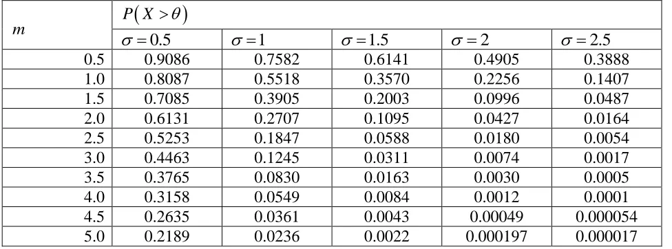
Table 1: Numerical values for Probability of disaster P X







for different values of mand 

m





P X  0.5

   1  1.5  2  2.5

0.5 0.9086 0.7582 0.6141 0.4905 0.3888 1.0 0.8087 0.5518 0.3570 0.2256 0.1407 1.5 0.7085 0.3905 0.2003 0.0996 0.0487 2.0 0.6131 0.2707 0.1095 0.0427 0.0164 2.5 0.5253 0.1847 0.0588 0.0180 0.0054 3.0 0.4463 0.1245 0.0311 0.0074 0.0017 3.5 0.3765 0.0830 0.0163 0.0030 0.0005 4.0 0.3158 0.0549 0.0084 0.0012 0.0001 4.5 0.2635 0.0361 0.0043 0.00049 0.000054 5.0 0.2189 0.0236 0.0022 0.000197 0.000017

Alternatively we may also obtain the values of mfor fixed values of  at different tolerance level from the equation.

1 1

( 1)

m

m e 

 

  

 

 _   _

  

1 1

( 1) m

e   m



 

 

 _   _

  

for 0.5,we get the expression for

 

0.5

1 3

m m

[image:3.612.65.553.178.359.2]

f m e   (2.5) Here, the equation (2.5) is a nonlinear equation and hence solved by Newton Raphson method for different real values of m using Mathematica Software.

Table: 2 Values of

m

for tolerance levels



and for  0.5

 0.1 0.05 0.02 0.01 0.001 0.0001 0.00001

(4)

Remarks:

1. Table 1 depicts the probability of disaster for Shushila distributed stress. It is interested to note that theprobability of disaster decreases for increasing values of m and decreases for the increasing values of  .

2. Table 2 shows the values of mfor different values of  for fixed  0.5.It is obvious that values of mincreases as decreases i.e. the ultimate strength capacity must increase if we wish to have a small tolerance level.

3 Stress and Strength-Reliability

For the stress strength model the probability PPr



Y X



when the random variable X and Y follows pdfs

 

1.1 and

 

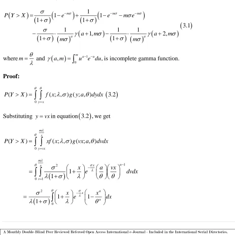
1.2 , respectively is given by the following theorem.

Theorem 3.1:PPr



Y  X



is given by



  















  



     



1

1 1

1 1 1

1, 2,

1 1

m m m

a a

P Y X e e m e

a m a m

m m

  

 _

 

 _ _ _ _

   

  

     

 

     

 

 

3.1

wherem 



 and





1

0

, m a u ,

a m u e du

 _  



is incomplete gamma function.

Proof:

0

( ) ( ; , ) ( ; , ) y x

P Y X f x g y a dydx

 

  



 

 

 

3.2

Substituting yvxin equation

 

3.2 , we get

0

( ) ( ; , ) ( ; , ) m

x

y vx

P Y X xf x g vx a dvdx 



  



 

 





1 2

0 1

1 1

m

a x

x

v

x a vx

e dvdx



 

 

    

 



    

 _  _ _{ } _

     

 





2

0

1 1

1

a x

a

x x

e dx

 

 

   

  

 

 _  _ _  _

[image:4.612.66.529.266.729.2]

(5)

settingm   





2 0 1 1 1

m _x a

a a x x e dx m               _  _ _  _ 



   





2 0 0 1 1 1

m _x m a

a a

x x x

e dx dx

m                 _  _  _  _ 



 



 

















2 2 2

0 0 0

2

1 0

1

1 1 1

1 1

m m m

x x _a x

a a m x a a a x

e dx e dx x e dx

m

x e dx m                                          







P Y  X   I II IIIIV

Now Integral is given by





2 0 1 m x

I e dx

        





1



1

m

I  e 

     _  _ 





2 0 1 m x x

II e dx

         





1 1





1



m m

II e  m e 

      





2 0 1 1 m x a a a

III x e dx

m           



Using Incomplete gamma function

 

1

0

, x

a t

a x t e dt

 _  







2 1 1 1 1 0 1 1 m a a t

a a a

III t e dt

(6)



1

  

1 a



1,



III a m

m

 _ _

 _

  





1

  

1 a



1,



III a m

m

 _ _

 

  







2

1 0

1 1

m

x a a a

IV x e dx

m

 

  

 

 







11



1



2,



a a a

IV a m

m

 _ _

  

 

  _{ }  

  

so we get





P Y X   I II IIIIV

Therefore,



  





 







  





 





1

1 1

1

1 1

1, 2,

1

m m m

a

P Y X e e m e

a m a m

m

  

 



   

 _

  

     



   



 

3.3

Hence, the theorem follows.

Table: 3 Strength-Reliability of an item for selected values of m and

a

for  1.5

m

a





2 3 4 5 6

(7)

Remarks:

1. Table 3 shows that the strength reliability of an item is increasing when we increase the values of m accordingly. If we increase the parametric values of power function i.e. “a”, the strength reliability of the system also increases.

Reference:

1. Awad, A.M. and Gharraf, M.K. (1986): Estimation of P(Y<X) in the burr case, A comparative study. Comm. Statist. B- Simulation comput., 15(2), 389-403.

2. Alam and Roohi (2003): On facing an exponential stress with strength having power function distribution. Aligarh J. statist., 23, 57-63.

3. Church, J.D. and Harries, B. (1970): The estimation of reliability from stress-strength relationships. Technometrics, 12,49-54.

4. Chao, A. (1982): On comparing estimators of P(X>Y) in the exponential case. IEEE Trans. Reliability, R-26, 389-392.

5. Chaturvedi, A. and Surinder, K. (1999): Further remarks on estimating the reliability function of exponential distribution under type-I and tyoe-II censoring. Brazilian Jour. Prob. Statist., 13. 29-39.

6. Downton, F. (1973): The estimation of Pr(Y<X) in the normal case. Technometrics, 15, 551-558.

7. Kelly, G.D., Kelly, J.A. and Schucany, W.R. (1976):Efficient estimation of P(Y<X) in the exponential case. Technometrics, 18, 359-360.

8. Sathe, Y.S. and Shah, S.P. (1981): On estimating P(X<Y) for the exponential distribution. Commun. Statist. Theor. Meth., A10, 39-47.

9. Shankar, R., Sharma S., Shankar, U. and Shankar, R., (2013): Shushila distribution and its application to waiting times data. Int. J. Bus. Manag., 3, 01-11.