Bayesian Analysis

Print Publication Date: Aug 2008

Subject: Political Science, Political Methodology, Comparative Politics

Online Publication Date: Sep 2009

DOI: 10.1093/oxfordhb/9780199286546.003.0021

Bayesian Analysis

Andrew D. Martin

The Oxford Handbook of Political Methodology

Edited by Janet M. Box-Steffensmeier, Henry E. Brady, and David Collier

Oxford Handbooks Online

Abstract and Keywords

This article surveys modern Bayesian methods of estimating statistical models. It first provides an introduction to the Bayesian approach for statistical inference, contrasting it with more conventional approaches. It then explains the Monte Carlo principle and reviews commonly used Markov Chain Monte Carlo (MCMC) methods. This is followed by a practical justification for the use of Bayesian methods in the social sciences, and a number of examples from the literature where Bayesian methods have proven useful are shown. The article finally provides a review of modern software for Bayesian inference, and a discussion of the future of Bayesian methods in political science. One area ripe for research is the use of prior information in statistical analyses. Mixture models and those with discrete parameters (such as change point models in the time-series context) are completely underutilized in political science.

Keywords: Bayesian method, Markov Chain Monte Carlo methods, software, statistical models, social sciences, political science

1 Introduction

Since the early 1990s, Bayesian statistics and Markov Chain Monte Carlo (MCMC) methods have become

increasingly used in political science research. While the Bayesian approach enjoyed philosophical cachet up until that point, it was impractical (if not impossible) for applied work. This changed with the onset of MCMC methods, which allowed researchers to use simulation to fit otherwise intractable models. This chapter begins with an introduction to the Bayesian approach for statistical inference, contrasting it with more conventional approaches. I then introduce the Monte Carlo principle and review commonly used MCMC methods. This is followed by a practical justification for the use of Bayesian methods in the social sciences, and a number of examples from the literature where Bayesian methods have proven useful. The chapter concludes with a review of modern software for Bayesian inference, and a discussion of the future of Bayesian methods in political science.

(p. 495) 2 The Bayesian Approach

The Bayesian approach to statistical inference begins at the same place as more conventional approaches: a probability model (also known as a data‐generating process). A probability model relates observed data y to a set of unknown parameters θ, with the possible inclusion of fixed, known covariates x. Our data are usually a

collection of observations indexed i = 1,…, n: y = {y , y ,…, y }. The observed data need not be scalars; in fact, they can be anything supported by the probability model, including vectors and matrices. The probability model has k parameters, which are represented θ = (θ , θ …, θ ). The covariates, or independent variables, are typically a collection of column vectors: x = {x , x ,…, x }. The probability model can be written f(yǀθ, x), or suppressing the conditioning on the covariates, f(yǀθ). It is important to stress the importance of choosing

1 2 n

1 2 k

appropriate probability models. While canonical models exist for certain types of dependent variables, the choice of model is rarely innocuous, and is thus something that should be tested for adequacy.

The linear regression model is, perhaps, the most commonly used probability model in political science. Our dependent variable y = {y , y ,…, y } is a collection of scalars with domain y ∊ ℝ. Our independent variables can be represented as a collection of column vectors x = {x , x ,…, x }, each of dimension (K × 1). We typically assume that the conditional distribution of y given x is normal:

This distributional assumption, along with an assumption that the observations are independent, yields a probability model with two parameters: θ = {β, σ }. β is a (K×1) vector that contains the intercept and slope parameters; σ is the the conditional error variance. The probability model for the linear regression model is thus

I will use this probability model as an illustration throughout this chapter.

The purpose of statistical inference is to learn about parameters that characterize the data‐generating process given observed data. In the conventional, frequentist approach to statistical inference, one assumes that the parameters are fixed, unknown quantities, and that the observed data y are a single realization of a repeatable process, and can thus be treated as random variables. The goal of the frequentist approach is to produce estimates of these unknown parameters. These estimates are denoted θ̑. The most common way to obtain these estimates is by the method of maximum likelihood (for an introduction to this method for political scientists, see King 1989). This method uses the same probability model, but treats it as a function (p. 496) of the fixed, unknown parameters. For our regression example:

One maximizes the likelihood function ℒ,(∙) with respect the parameters to obtain the maximum likelihood estimates; i.e. the parameter values most likely to have produced the observed data. To perform inference about the

parameters, the frequentist recognizes that the estimated parameters θ̑ result from a single sample, and uses the sampling distribution to compute standard errors, perform hypothesis tests, construct confidence intervals, and the like.

When performing Bayesian inference, the foundational assumptions are quite different. The unknown parameters θ are treated as random variables, while the observed data y are treated as fixed, known quantities. (Both the Bayesian and frequentist approach treat the covariates x as fixed, known quantities.) These assumptions are much more intuitive; the unobservable parameters are treated probabilistically, while the observed data are treated deterministically. Indeed, the quantity of interest is the distribution of the parameter θ after having observed the data y. This posterior distribution can be written f(θǀy), and can be computed using Bayes's Theorem:

The posterior distribution is the conditional distribution of the parameters after having observed the data (as opposed to the prior, which is that distribution before having observed the data). The posterior is a formal, probabilistic statement about likely parameter values after observing the data. Bayes's Theorem follows directly from the axioms of probability theory, and is used to relate the conditional distributions of two variables.

One of the three quantities on the right‐hand side of equation (4) is familiar: f(yǀθ) is the likelihood function dictated by the probability model. (The likelihood function plays a crucial role in both frequentist and Bayesian approaches to data analysis; what is done with the likelihood function is what differs between the two approaches.) The second expression in the numerator f(θ) is called the prior distribution. This distribution contains all ex ante information about the parameter values available to the researcher before observing the data. Often researchers use noninformative (or minimally informative parameters) such that the amount of prior information included in the analysis is small. The denominator of equation (4) contains the prior predictive distribution:

1 2 n i

1 2 n

i i

While this quantity is useful in some settings, such as model comparison, most of the time researchers work up to a constant of proportionality, f(θǀy) α f(yǀθ)f(θ).

The posterior distribution, in essence, translates the likelihood function into a proper probability distribution over the unknown parameters, which can be (p. 497) summarized just as any probability distribution; by computing expected values, standard deviations, quantiles, and the like. What makes this possible is the formal inclusion of prior information in the analysis. For accessible introductions to Bayesian methods see the textbooks by Gill (2002) and Gelman et al. (2004), or the expository articles by Jackman (2000; 2004).

To perform Bayesian inference for the linear regression model, we need to include prior information about our two parameters. These priors can take any form, and are completely at the discretion of the analyst. For the sake of illustration, suppose that β and σ are a priori independent, with the prior information about β encoded in a multivariate normal distribution

, and prior information about the inverse of the conditional error variance in a Gamma distribution σ ~ gamma(c /2, d /2). For any application, the analyst would choose values of the hyperparameters b , B , c /2, and d /2 that characterize the prior distribution. These priors result in a posterior distribution for the linear regression model:

where f(β) is the multivariate normal density, and f(σ ) is a Gamma density. Getting from a probability model to the posterior distribution is an exercise in taking a probability model, deriving the likelihood function, and positing probabilistic prior beliefs.

So why have Bayesian statistics not been widely used in political science until very recently? Writing down a posterior distribution is a straightforward algebraic exercise, but summarizing the distribution is far more complicated. To compute something as simple as the posterior expected value requires integrating the posterior distribution which, except for the most trivial of models, is analytically impossible. We thus require computation methods to summarize posterior distributions, which leads us to simulation methods.

3 Model Fitting via Simulation

Analytically summarizing posterior distributions is typically impossible. Over the last twenty years, Bayesian statisticians have harnessed the Monte Carlo method (Metropolis and Ulam 1949) to perform this summarization numerically. While these methods can be employed to study any distribution, the discussion here will focus solely on Monte Carlo methods commonly used in Bayesian statistics. We are interested in learning about the posterior distribution, f(θǀy), which I will call the target distribution because it is the distribution from which we intend to simulate. (There are other distributions we might be interested in simulating from, including the posterior and prior predictive distributions.) The Monte Carlo method is based (p. 498) on a simple idea: One can learn anything about a target distribution by repeatedly drawing from it and empirically summarizing those draws. For example, we might be interested in computing the posterior expected value, which can be done analytically by computing a high‐dimensional integral:

If we were able to produce a random sequence of G draws θ ,θ ,…,θ ) from f(θǀy), we could approximate the posterior expected value by taking the average of these draws:

The precision of the estimate depends solely on the quality of the algorithm employed, and the number of draws taken from the target distribution (which is only limited by the speed of one's computer and one's patience). Similar methods can be used to compute the posterior standard deviation or quantiles, probabilities that parameters take particular values, and other quantities of interest. What all of these methods have in common is that they serve to compute high‐dimensional integrals using simulation. A great deal of work in numerical analysis is devoted to

2

−2

0 0 0 0 0 0

−2

understanding the properties of algorithms; for such a discussion of commonly used methods in Bayesian statistics, see Tierney (1994).

To use the Monte Carlo method to summarize posterior distributions, it is necessary to have algorithms that are well suited to producing draws from commonly found target distributions. Two algorithms—the Gibbs sampling and Metropolis— Hastings algorithms—have proven to be very useful for applied Bayesian work. Both of these algorithms are Markov Chain Monte Carlo methods, which means that the sequence of draws θ , θ ,…, θ ) are dependent; each draw θ ) depends only on the previous draw θ . The sequence of draws thus forms a Markov chain. Algorithms are constructed such that the Markov Chain converges to the target density (its steady state) regardless of the starting values.

Click to view larger

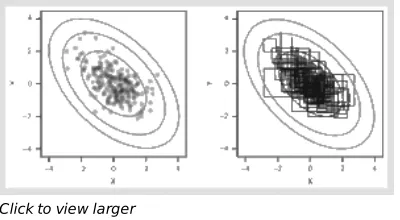
Fig. 21.1. An illustration of Gibbs sampling from a bivariate normal distribution

Note: The target distribution is represented by the grey contour lines. Each cell depicts 200 draws after 100

burn‐in iterations, which are discarded. The left‐hand cell depicts the individual draws; the right‐hand cell shows the trajectory of the sampler.

The Gibbs sampling algorithm (Geman and Geman 1984; Gelfand and Smith 1990) uses a sequence of draws from conditional distributions to characterize the joint target distribution. Suppose that our parameter vector θ has three components, making our target distribution f(θ , θ , θ ǀy). To use the Gibbs sampler, one begins by choosing starting values

and

(starting values are usually chosen near the posterior mode or the maximum likelihood estimates). One then repeats, for g = 1,…, G iterations (making sure to store the sequence of draws at each iteration):

(p. 499)

Since we are always conditioning on past draws, the resultant sequence results in a Markov Chain. When computing Monte Carlo estimates of quantities of interest, like the posterior mean, one discards the first set of “burn‐in” iterations to ensure the chain has reached steady state. For the posterior distribution of many common models, these conditional distributions take known forms; e.g. multivariate normal, truncated normal, Gamma, etc. So, while the joint posterior distribution is difficult to simulate from directly, it is easy to simulate from these conditionals.

To illustrate the Gibbs sampling algorithm in practice, Figure 21.1 shows sampling from a bivariate normal

distribution f(X, Y), where both X and Y have mean 0 and variance 1, and cov(X, Y) = −0.5. The sampler iteratively draws YǀX and then XǀY from the conditional distributions, each of which take the following form for this example:

f(YǀX) = N(−0.5X, 0.75). What is apparent in Figure 21.1 is that the sampler seems to be sampling from the proper

target distribution. The trajectory of the sampler takes a city block pattern because X and Y are updated sequentially. See Casella and George (1992) for an accessible introduction to Gibbs sampling.

(1) (2) (G)

(g+1) (g)

Click to view larger

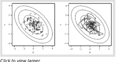
Fig. 21.2. An illustration of an ill‐conditioned Metropolis—Hastings sampler with a uniform random walk

proposal from a bivariate normal distribution

Note: The target distribution is represented by the grey contour lines. Each cell depicts 200 draws after 100

burn‐in iterations, which are discarded. The left‐hand cell depicts the individual draws; the right‐hand cell shows the trajectory of the sampler.

The second algorithm that enjoys common use in applied Bayesian statistics is the Metropolis‐Hastings algorithm, first introduced by Metropolis et al. (1953) and generalized by Hastings (1979). Chib and Greenberg (1995) provide an accessible introduction to this algorithm. The algorithm has many applications beyond Bayesian statistics; it is commonly used for all sorts of numerical integration and optimization. (It is also the case that the Gibbs sampling algorithm is a special case of the Metropolis‐Hastings algorithm.) To simulate from our target distribution f(θǀy), we again start with sensible starting values: θ . For each iteration of the simulation g = 1,…, G, we draw a proposal θ* from a known proposal distribution p (θ*ǀθ ). One chooses a proposal distribution from which it is easy to sample, (p. 500) such as a uniform distribution over a particular region, or a multivariate normal or multivariate‐t, centered at the current location of the chain, the posterior mode, or perhaps elsewhere. It is important to choose a proposal distribution such that the chain “mixes well;” i.e. adequately explores the posterior distribution. The convergence diagnostics, discussed below, can be used to determine how well the chain is mixing. For each iteration, we set

.

With a* defined:

Unlike the Gibbs sampling algorithm, when each move is automatically accepted, one accepts the proposal distribution probabilistically, sometimes moving to a value with a higher density value, sometimes moving to one with a lower density value. Just as with the Gibbs sampling algorithm, the steady state of the Markov chain

characterized by this algorithm is the target distribution, in this case the posterior distribution. Figure 21.2 illustrates sampling from the same bivariate normal distribution using Metropolis‐Hastings with a uniform random walk proposal with width of two units. In Figure 21.2 we see that this Metropolis—Hastings sampler traverses the space more more slowly; in fact, 30 percent of the time the sampler does not move at all. The size of the proposal distribution is also somewhat small, which keeps the sampler in certain parts of the distribution longer than a better conditioned sampler.

(p. 501) Without being able to plot the target distribution, which in most applications is of high dimension, it would be difficult, if not impossible, to assess whether the chain is sampling from the target distribution. An important part of any Bayesian analysis is assessing the convergence of the simulation results. Indeed, no Monte Carlo

estimates of posterior density summaries can be trusted unless the chain has reached its steady state. But just

as it is impossible to know, in most circumstances, that a numerical optimizer has reached the global maximum likelihood estimate, so too is it impossible to know for sure whether a Markov Chain Monte Carlo algorithm has converged. However, there are a number of methods that can be used to take output from a MCMC sampler and test whether the sequence of draws is consistent with convergence (see the review pieces by Cowles and Carlin 1995; Brooks and Roberts 1998). Each of these convergence diagnostics is based on one of a number of criteria; some look at the marginal posterior distributions to see if the traceplots are stationary (using a number of different tests). Others compare multiple runs from different starting values and using different random number seeds to

(0)

determine whether the chains converge in such a way as to make their different starting values irrelevant. It is important to note that finding nonconvergence of any parameter means that the entire chain has not converged, and it needs to be run longer (or reimplemented using a different algorithm). Every analyst should use these diagnostic tools before computing any posterior density summaries or reporting results, and results from these diagnostics should be presented in research papers.

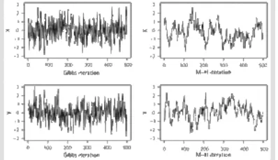
I present in Figure 21.3 the traceplots for both X and Y for the simulation results presented above. For this short‐run length of 500 iterations neither of these chains passes the standard battery of tests, but by inspection it is clear that the Gibbs sampler is mixing far better than the Metropolis—Hastings chain. A poor mixing chain traverses slowly through the parameter space, and the traceplots will show a close following pattern, as in the right‐hand cells of Figure 21.3. (The reader should not take the point that Gibbs sampling works well and Metropolis‐Hastings does not; this is solely a feature of the illustration). All of the standard tests for convergence are implemented in the coda (Plummer et al. 2005) package in the R language (R Development Core Team 2005).

4 Practical Advantages of Bayesian Methods

The Bayesian approach to data analysis requires a different set of assumptions and computational tools than the classical approaches typically used in political science. This section provides a number of practical advantages of performing Bayesian inference.

Click to view larger

Fig. 21.3. Marginal density traceplots of Gibbs and Metropolis—Hastings sampling from a bivariate normal

distribution

Note: These traceplots depict the same simulation results as Figures 21.1 and 21.1, except they depict 500

iterations after 100 burn‐in iterations.

(p. 502)

4.1 Intuitive Interpretation of Findings

In classical statistics hypothesis tests and confidence intervals are used to perform statisical inference. We choose to reject a null hypothesis when the probability of observing sample data as inconsistent or more inconsistent with a posited null hypothesis is quite low. At base, a rejected null hypothesis (and thus claiming “statistical

significance”) tells us that an effect exists. Confidence intervals are also used to provide a range of likely values for parameter estimates; i.e. they can be used to make claims about effect sizes. Precisely interpreting confidence intervals is a difficult proposition.

collected about, for example, institutions or markets.) In addition, most frequentist hypothesis tests and confidence intervals require the assumption of an infinitely large sample size. Such asymptotic assumptions are not necessary when using the Bayesian approach. Even if one is comfortable with the sample size and the ability to resample from the population, a confidence interval does not provide a probabilistic statement about parameter values.

This is quite different in the Bayesian context. It is straightforward to summarize the posterior and compute any number of interesting quantities, all of which can be treated as probabilities. Analogous in some ways to a frequentist p‐value, the Bayesian analyst can compute the probability that a parameter value is positive or negative. Akin to a confidence interval, one can also write down a range of values that contain the parameter value a certain percentage of the time. Unlike confidence intervals, these Bayesian credible intervals (which are typically computed using the highest posterior density region) can be interpreted probabilistically. A 95 percent Bayesian credible interval for θ of [3.2, 6.1] suggests that, after observing the data, there is a 95 percent chance that the parameter falls between 3.2 and 6.1. Computing these probabilities requires summarizing the posterior density, and is typically done using MCMC methods.

4.2 Quantities of Interest

When analyzing data, parameters of statistical models are typically not the quantities of interest. Indeed, we are typically interested in functions of parameters, such as predicted values (King, Tomz, and Wittenberg 2000). Using Bayesian methods makes it easy to compute many types of quantities of interest, and propagate the uncertainty about parameters into uncertainty about these quantities. One useful example is the posterior predictive distribution, which can be summarized to provide ranges of values for a new datapoint y :

Just as with Bayesian credible intervals, these intervals will also be on the scale of probability, and can be interpreted as such.

In the frequentist context, providing confidence intervals for quantities of interest is difficult for nearly all cases except the linear model. To compute these quantities analytically requires the use of the delta method, which can provide arbitrarily precise approximations. There are also simulation‐based approaches (King, Tomz, and

Wittenberg 2000). In the frequentist context, these intervals suffer the same ills as confidence intervals: They are based on assumptions that the sample size is infinite (such that the sampling distribution is multivariate normal; King, Tomz, and Wittenberg 2000, 352), and require the logic of repeated sampling which is implausible in many political science applications.

(p. 504) The quantities over which one can compute probabilities are limited only by the creativity of the researcher. In the context of estimating latent ideal points for Supreme Court justices, Jackman argues how MCMC methods can be used to perform inference for “comparisons of ideal points, rank ordering the ideal points, the location of the median justice, cutting planes for each bill (or case), residuals, and goodness‐of‐fit summaries” (Jackman 2004, 499). All of these quantities of interest can be computed using MCMC methods.

4.3 Incorporation of Prior Information

Political scientists typically have a great amount of substantive knowledge gleaned from the political science literature, fieldwork, and journalistic accounts. One advantage of Bayesian methods is the ability to formally include this type of information in a statistical analysis through the use of informative priors. (Related to this is the ability to include results from previous statistical studies by repeatedly using Bayes's Rule, or combining results from a number of studies using meta‐analysis.) Western and Jackman (1994) argue that this strategy is particularly germane to the study of comparative politics, where sample sizes are quite low (and, thus, asymptotic properties of estimators have likely not yet kicked in). Translating rich, substantive information into statements about parameters of probability models is a difficult task. Gill and Walker (2005) review the prior elicitation literature, and use some of these tools to translate expert opinion into priors on the marginal effects of various covariates on attitudes toward the judiciary in Nicaragua. One does not need to use informative priors when doing Bayesian inference; indeed, much applied work uses so‐called “uninformative” priors, which bring little, if any, information into the analysis. It is important to keep in mind that when using informative priors it is necessary to perform sensitivity analysis to ensure

that the prior beliefs are not unduly affecting the results.

4.4 Fitting Otherwise Intractable Models

When performing classical inference, numerical optimatization is the computational method used to fit models; one finds parameter values by maximizing some function, in most cases a likelihood function. Bayesian inference, on the other hand, has integration at its core. There are a number of examples where MCMC methods afford the opportunity to fit models that are otherwise difficult, if not impossible, to fit using conventional methods.

Quinn, Martin, and Whitford (1999) use MCMC methods to fit multinomial probit models (MNP) of voter choice in the Netherlands and the UK. These models, which allow for correlated errors in the latent utility specification, are difficult to fit using classical approaches because of the high‐dimensional integrals one needs to compute to evaluate the likelihood function (also see the strategic censoring model (p. 505) of Smith 1999). Another example are measurement models, such as the item response model used to uncover ideal points in legislatures (Clinton, Jackman, and Rivers 2004), or the dynamic item response theory model of Martin and Quinn (2002), which allows smooth evolution of ideal points when dealing with multiple cross‐ sections of data. These models are difficult in the classical context because the number of parameters grows with each additional legislator or bill.

Bayesian methods are also extremely promising in dealing with data that are organized hierarchically. Western (1998) models some cross‐sectional time‐series data using Bayesian methods. Working with these data in a classical context is difficult because either the number of clusters (e.g. multivariate time‐series data), time periods (e.g. panel data), or both (e.g. cross‐sectional time‐series data as typically used in comparative and international political economy) are small. This does not cause any difficulty in the Bayesian context, which can be modified to deal with other types of complex dependence.

There are also some models that have discrete parameters, which are difficult to deal with in the classical context because the optimization problem is not continuous. One example would be estimating the number of mixture components or the number of dimensions in a latent space model. Green (1995) provides an algorithm suited to these types of problems called reversible jump MCMC. In the time‐series context, we might be interested in

estimating the number and location of structural breaks in the data. The methods of Chib (1998) are suited to these change point models. In all of these cases, adopting a Bayesian approach and using MCMC for model‐fitting opens doors to new types of analyses.

4.5 Model Comparison

Political scientists are typically engaged in comparing explanations of political phenomena. Different explanations often dictate very different models of the observed data y. The Bayesian approach to statistical inference offers an extremely useful tool for model comparison called Bayes' factors (Kass and Raftery 1995). Bayes' factors can be used to compare models with different blocks of covariates, models with different functional forms, and can be used with any number of plausible models (because transitivity holds in all pairwise comparisons). As with all quantities in the Bayesian approach, Bayes' factors provide the posterior probability that model M is the true data‐ generating process compared with model M . Since each model contains prior information about the parameters of the model, Bayes' factors are sensitive to the priors chosen. The quantities used to compute Bayes' factors are the prior predictive distribution (see equation (5)), and the prior probabilities assigned to each model (typically one assumes that each model is a priori equally likely). Quinn, Martin, and Whitford (1999) use Bayes' factors to

compare two different theoretical models and two different functional forms (multinomial probit and multinomial logit) in their comparative voting study. For an accessible introduction to Bayes' factors for a social science audience see Raftery (1995).

(p. 506) Computing the prior predictive distribution is a difficult task. While there exist MCMC methods that can be used in some situations, others have developed model comparison heuristics that are far easier to compute, such as the Bayesian Information Criterion (Raftery 1995) or the Deviance Information Criterion (Spiegelhalter et al. 2002), which is computed automatically in the WinBUGS software package.

4.6 Missing Data

Missing data is a common problem in political science, and is easily taken into account in the Bayesian context by using data augmentation (Tanner and Wong 1987). Data augmentation works by using the data‐generating process as an imputation model. As such, it is easy to estimate models when some of the data y are missing. Not only will the recovered estimates take into account the uncertainty caused by the missing data, but the analyst can access the imputed values, which will average over all parameter uncertainty when producing the values. What about missing data in the covariates x? This is a more difficult problem, because in both the frequentist and Bayesian context the covariates are assumed to be fixed and known. However, given an imputation model for the missing covariates, it is straightforward to adapt an MCMC algorithm to average over the missing covariate information when performing inference about parameters and quantities of interest. The software package WinBUGS automatically performs data augmentation for all missing data y.

4.7 Common Concerns

While there are a number of practical advantages of using Bayesian methods in political science, there are some common concerns, which I detail below with some reactions.

• Bayesian analysis is far more complicated than classical statistics. The mathematics that underlie Bayesian

methods are no more complicated than those needed to perform classical inference. MCMC algorithms are no more complicated that the numerical optimization and matrix inversion routines. The unfamiliar will always appear more complex than the familiar.

• Priors are subjective, and they can be used to drive results. It is true that priors are subjective; but so too

are any number of assumptions, including what model to use, what covariates to include or exclude in the analysis, and in what fashion they should relate to the dependent variable. All of these modeling choices are, in a sense, subjective. What is of utmost importance is to test all testable assumptions in order to determine which model is best. Bayes' factors are particularly useful in this light. Also, as long as one performs prior sensitivity analysis, it is possible to determine whether the prior or the data are driving results. Simply put, if changing the prior changes the posterior, the data are not informative about the parameter values and the priors are driving the results. Such sensitivity analysis should be an important part of any applied Bayesian work.

(p. 507)

• There is no way to know whether an MCMC algorithm has converged. This is true. However, there are

diagnostics, discussed above, which can be used to determine nonconvergence (Cowles and Carlin 1995; Brooks and Roberts 1998). In the classical context, there is also no way to know whether a numerical optimization algorithm has reached a global maximum in most cases.

• There is no good software to perform Bayesian inference. There exists no widely used statistical software for

Bayesian inference that compares to commercial products such as SAS, SPSS, or Stata. (This is likely due to the fact that all of these packages were developed before MCMC methods were widely used.) Over the last decade a number of promising software packages have emerged, which I discuss in the following section.

5 Software

Until the late 1990s, those interested in doing applied Bayesian work needed to develop their own MCMC algorithms and write their own software. Much of this work was done in high‐level languages like GAUSS, Matlab, R, or S‐Plus, or low‐level languages like FORTRAN or C. The ability to develop these algorithms and produce software remains an important skill for the applied analyst, as existing software packages are limited in their scope. (It is also the case that developing software is an important part of innovation for those working in the classical paradigm.)

Today there exist two different types of software packages useful for Bayesian inference. The first is the BUGS language. BUGS stands for Bayesian updating using Gibbs sampling. To use BUGS, one writes down a model definition using an R‐like syntax. The model definition is then processed, and the program chooses a scheme to sample from the posterior distribution of the model. Here is an example of BUGS syntax for our linear regression model with semi‐conjugate priors:

3   Y[i] ̃ dnorm(mu[i],tau) 4    mu[i] ← inprod(X[i,], beta) 5   }

6

7  for(k in 1:K) {

8   beta[k] ̃ dnorm(0,0.001) 9  }

10  tau ̃ dgamma(0.001, 0.001) 11  }

The first five lines of the code define the probability model. Here each observation y is assumed to be distributed conditionally normal with a common precision (inverse (p. 508) variance) τ. Lines 7–10 define the priors, in this case univariate normal for each element of the β, and Gamma for the precision. With this model definition and some data, the BUGS language will use MCMC methods to sample from the posterior. The most commonly used BUGS implementation is the WinBUGS package, which runs only on Microsoft Windows machines (Spiegelhalter et al. 2004). There are two newer implementations of the BUGS language: OpenBUGS (Thomas 2004) which runs on the Linux operating system, and JAGS (Plummer 2005) which is platform independent. The BUGS language works well for most simple models.

The second option is to use contributed software to the R language (R Development Core Team 2005). There are a number packages that are useful for performing applied Bayesian inference. Two general packages that provide model estimation for a number of commonly used models are MCMCpack (Martin and Quinn 2005) and bayesm (Rossi and McCulloch 2005). MCMCpack, for example, uses common R syntax to specify models. Consider the following example code used to fit a linear regression model:

The returned object posterior is an mcmc object which can be summarized using the coda package (Plummer et al. 2005). Prior information is included in the model by passing hyperparameter arguments to the model fitting function. The “Bayesian Task View” on the Comprehensive R Archive Network (<http://cran.r-project.org>) contains

information about many more packages, including those that fit single models or single classes of models, that are available for the R language.

6 Conclusion

Bayesian methods and estimation via Markov Chain Monte Carlo afford a number of advantages to applied political scientists. The methods can be applied in many situations to answer all sorts of substantive questions. Most importantly, all quantities of interest, including parameter estimates, can be stated as probabilities, and as such comport with the manner in which we typically think about estimation.

I conclude this chapter with some thoughts about places for future research, and for promising applications. One area ripe for research is the use of prior information in statistical analyses. Prior elicitation is an underdeveloped field, and there are elicitation problems unique to the study of politics, such as encoding elite opinion or attitudes, or information produced by governmental agencies. Developing new methods for translating that information into formal statements about parameters seems like a promising field of research. So, too, are guidelines for sensitivity analysis. When using informative priors, political scientists need guidance as to testing the (p. 509) dependence of the findings on the included prior information. Another area that needs significant work is statistical software. While the BUGS language and various R packages are promising, there is not yet a lingua franca for applied Bayesian work. This lack of available software makes doing Bayesian work more difficult than it otherwise should be. Finally, there are a number of models and methods that are wholly underutilized in political science that I think exhibit great promise. These include mixture models, and those with discrete parameters (such as change point models in the time‐series context). Formal model comparison is also rarely performed in political science. Bayes' factors provide an avenue to comparing many different types of models. When dealing with clustered data, such as cross‐sectional time‐series data, hierarchical models show great promise. These models are easily fit using MCMC, and can be extended to handle many different types of complex dependence. Just as with any statistical tool, Bayesian methods are limited only by the creativity of the practitioner, yet to date the advantages of Bayesian

methods have not yet been fully explored in political science.

References

BROOKS, S. P. and ROBERTS, G. O. 1998. Assessing convergence of Markov chain Monte Carlo algorithms. Statistics and Computing, 8: 319–35.

CASELLA, G. and GEORGE, E. I. 1992. Explaining the Gibbs sampler. American Statistician, 46: 167–74.

CHIB, S. 1998. Estimation and comparison of multiple change‐point models. Journal of Econometrics, 86: 221–41.

—— and GREENBERG, E. 1995. Understanding the Metropolis—Hastings algorithm. American Statistician, 49: 327–36.

CLINTON, J. D. JACKMAN, S. and RIVERS, D. 2004. The statistical analysis of roll call data. American Political Science Review, 98: 355–70.

COWLES, M. K. and CARLIN, B. P. 1995. Markov Chain Monte Carlo diagnostics: a comparative review. Journal of the American Statistical Association, 91: 883–904.

GELFAND, A. E. and SMITH, A. F. M. 1990. Sampling‐based approaches to calculating marginal densities. Journal of the American Statistical Association, 85: 398–409.

GELMAN, A. CARLIN, J. B. STERN, H. S. and RUBIN, D. B. 2004. Bayesian Data Analysis, 2nd edn. Boca Raton, Fla.:

Chapman and Hall/CRC.

GEMAN, S. and GEMAN, D. 1984. Stochastic relaxation, Gibbs distributions, and the Bayesian restoration of images. IEEE Transactions of Pattern Analysis and Machine Intelligence, 6: 721–41.

GILL, J. 2002. Bayesian Methods: A Social and Behavioral Sciences Approach. Boca Raton, Fla.: Chapman and

Hall/CRC.

—— and WALKER, L. D. 2005. Elicited priors for Bayesian model specifications in political science research. Journal of Politics, 67: 841–72.

GREEN, P. J. 1995. Reversible jump Markov Chain Monte Carlo computation and Bayesian model determination. Biometrika, 82: 711–32.

HASTINGS, W. K. 1979. Monte Carlo sampling methods using Markov Chains and their applications. Biometrika, 57:

97–109.

JACKMAN, S. 2000. Estimation and inference via Bayesian simulation: an introduction to Markov Chain Monte Carlo. American Journal of Political Science, 44: 369–98.

—— 2004. Bayesian analysis for political research. Annual Reviews of Political Science, 7: 483–505.

KASS, R. E. and RAFTERY, A. E. 1995. Bayes factors. Journal of the American Statistical Association, 90: 773–95.

KING, G. 1989. Unifying Political Methodology: The Likelihood Theory of Statistical Inference. Cambridge:

Cambridge University Press.

——  TOMZ, M. and WITTENBERG, J. 2000. Making the most of statistical analyses: improving interpretation and

presentation. American Journal of Political Science, 44: 341–55.

MARTIN, A. D. and QUINN, K. M. 2002. Dynamic ideal point estimation via Markov Chain Monte Carlo for the U.S.

Supreme Court, 1953–1999. Political Analysis, 10: 134–53.

——  ——2005. MCMCpack: Markov Chain Monte Carlo (MCMC) Package. R package version 0.6‐3. <>

METROPOLIS, N. and ULAM, S. 1949. The Monte Carlo method. Journal of the American Statistical Association, 44:

——  ROSENBLUTH, A. W. ROSENBLUTH, M. N. TELLER, A. H. and TELLER, E. 1953. Equation of state calculations by fast

computing machines. Journal of Chemical Physics, 21: 1087–92.

PLUMMER, M. 2005. JAGS: Just Another Gibbs Sampler. Version 0.8. <>

——  BEST, N. COWLES, K. and VINES, K. 2005. coda: Output Analysis and Diagnostics for MCMC. R package version

0.9‐2. <>

QUINN, K. M. MARTIN, A. D. and WHITFORD, A. B. 1999. Voter choice in multi‐party democracies: a test of competing

theories and models. American Journal of Political Science, 43: 1231–47.

R DEVELOPMENT CORE TEAM 2005. R: A Language and Environment for Statistical Computing. R Foundation for

Statistical Computing, Vienna. <>

RAFTERY, A. 1995. Bayesian model selection in social research. Sociological Methodology, 25: 111–96.

ROSSI, P. and MCCULLOCH, R. 2005. bayesm: Bayesian Inference for Marketing/Micro‐ econometrics. R package

version 2.0–1.

SMITH, A. 1999. Testing theories of strategic choice: the example of crisis escalation. American Journal of Political Science, 43: 1254–83.

SPIEGELHALTER, D. J. BEST, N. G. CARLIN, B. P. and VAN DER LINDE, A. 2002. Bayesian measures of model complexity and

fit. Journal of the Royal Statistical Society, B, 64: 583–639.

THOMAS, A. BEST, N. and LUNN, D. 2004. WinBUGS. Version 1.4.1. <‐ bsu.cam.ac.uk/bugs/winbugs>

TANNER, M. A. and WONG, W. 1987. The calculation of posterior distributions by data augmentation. Journal of the American Statistical Association, 82: 528–50.

THOMAS, A. 2004. OpenBUGS. <>

TIERNEY, L. 1994. Markov Chains for exploring posterior distributions. Annals of Statistics, 22: 1701–62.

WESTERN, B. 1998. Causal heterogeneity in comparative research: a Bayesian hierarchical modelling approach. American Journal of Political Science, 42: 1233–59.

—— and JACKMAN, S. 1994. Bayesian inference for comparative research. American Political Science Review, 88:

412–23.

Notes:

This research is supported by the National Science Foundation Methodology, Measurement, and Statistics Section, Grant SES-03-50646. I acknowledge Jong Hee Park, Kyle Saunders, and seminar participants at the University of South Carolina and the University of California, Davis, for their constructive comments about this chapter. R code to replicate the figures will be made available on the author's website <http://adm.wustl.edu>.

Andrew D. Martin