Maximum Pseudo-Likelihood Estimation
Minimizes Conditional Description Length
Matthew G. Reyes
∗David L. Neuhoff
†∗
self-employed †EECS Dept., University of Michigan
[email protected] [email protected]
Abstract—In this paper we discuss a method, which we call Minimum Conditional Description Length (MCDL), for estimating the parameters of a subset of sites within a Markov random field. We assume that the edges are known for the entire graph G= (V, E). Then, for a subset U ⊂V, we estimate the parameters for nodes and edges inU as well as for edges incident to a node in U, by finding the exponential parameter for that subset that yields the best compression conditioned on the values on the boundary∂U. Our estimate is derived from a temporally stationary sequence of observations on the setU. We discuss how this method can also be applied to estimate a spatially invariant parameter from a single configuration, and in so doing, derive the Maximum Pseudo-Likelihood (MPL) estimate.
I. INTRODUCTION
A Markov random field (MRF), also referred to as a Gibbs distribution, is a probability distribution on the colorings of an undirected graph G= (V, E), where the nodes1 inV are the random variable indices and the edges in E represent direct dependencies between the random variables [20]. One of the primary research areas for MRFs is the problem of model selection or parameter estimation, where the objective may either be to determine the parameters for known edges [1], determine the edges of the graph [8], or jointly find the edges and the parameters for those edges [13]. Markov fields are a natural class of models for many types of data, including images and social networks. In images, it is natural to assume a set of edges, for instance, those connecting the 4 or 8 nearest neighbors. And for social networks, neighbor relations are known. With these two applications in mind, this paper focuses on the first model selection problem, that of determining the parameters on known edges.
A family of MRFs is specified by a vector statistic t = (ti, i∈V;ti,j,{i, j} ∈E)defined on the site values at
indi-vidual nodes and the endpoints of the edges E of the graph.2 A particular MRF is indexed by an exponential parameter vector θthat scales the corresponding components oftin the probability of a configuration x, which is given by
p(x;θ) = exp{hθ, t(x)i −Φ(θ)}, (1) whereh,idenotes inner product andΦ(θ)is thelog-partition function.
In the model selection problem considered in this paper, the set of edgesEis known, as well as the statistict, and we have to determine the exponential parameter θ that weights
1We use the termsnodesandsitesinterchangeably.
2Properly, this is a pairwise MRF. Generalizations to other MRFs are straightforward.
the corresponding components of the statistic for nodes and edges. Generally, estimation is performed from a temporal sequence of observationsx1:n=∆x(1), . . . ,x(n), from which an estimate θˆn is obtained. While it is often assumed that the
x(i)are independent to simplify analysis, in fact it is sufficient to assume that x(1),x(2), . . .is stationary, which is what we assume in this paper.
A popular criterion for estimating a parameter within a family of candidate models is Maximum Likelihood (ML), which seeks the parameterθˆnwhich maximizes the probability
p(x1:n; ˜θ) of the observed data over all parameter vectors θ˜
indexing probability distributions within the specified class of probability distributions. For Markov fields, the ML criterion reduces to finding the exponential parameter θ˜such that the expected statisticµ˜=∆µ(˜θ)=∆Eθ˜[t(X)]under the MRF induced by θ˜, referred to as the moment of the MRF, equals the empirical moment µˆn of x1:n, which is the average value
1
n
Pn
i=1t(x
(i)) of the statistic from the n observations [10]. For a tractable graph, such as a tree or one that can be clustered into a tree with only moderate numbers of nodes per cluster, the moments can be exactly and efficiently determined with Belief Propagation (BP), an iterative message passing algorithm. Thus, one can compute moments {µ˜} for a set of candidates {θ˜} and choose the one whose moment µ˜
most closely matches the observed empirical moment µˆn.
For a general graph, however, BP is intractable and thus the momentµ˜cannot be computed exactly. This intractability can circumvented by approximating the momentµ˜, with either an approximate variant of BP [20], or by sampling the MRF’s corresponding to candidate θ˜, e.g. with Gibbs sampling [9], [10], [11], and selecting the θ˜ whose empirical moment µˆ˜
most closely matches that of the observed data.
expressed as a product of single-site conditional probabilities. Thus, by conditioning onxV\V1, one can estimateθthrough an
analytically tractable objective function. MPL extends this idea by finding the parameter θˆM P L that maximizes the
pseudo-likelihood function
PL(x; ˜θ) =
|V| Y
j=1
p(xj|xV\j; ˜θ)
over candidate parameters θ˜, or equivalently, the pseudo-log-likelihood function
logPL(x; ˜θ) =
|V| X
j=1
logp(xj|xV\j; ˜θ),
again assuming translation invariance, or spatial homogeneity, of t andθ. Again by the Markov property, these conditional probabilities simplify as conditional probabilities given the neighbors of each node. Much research has been done on MPL, and consistency of the MPL estimate θˆM P L has been
shown [12], [6]. An interpretation of MPL is that it finds the parameter θˆM P L such that the induced conditional
distribu-tions of individual nodes best match the empirical conditional distributions of individual nodes.
The parameter estimation method proposed in the present paper, which we call Minimum Conditional Description Length (MCDL), can be understood as a generalization of Maximum Pseudo-Likelihood. Whereas the MPL method es-timates a translation invariant parameter through observations
xU¯1, . . . ,xU¯n of n=|V|statistically identical subsets within a single observation x, we propose MCDL as a method for estimating the parameter θU¯ within a single subset U¯ from a sequence of observations x(1)U¯ , . . . ,x
(n) ¯
U on U¯, where ∂U
is the boundary or neighborhood of U and U¯ = U ∪∂U is the closure of U. We do not assume spatial homogeneity (translation invariance) of θ within G, but we do require temporal stationarity of x(1)U¯ , . . . ,x
(n) ¯
U . Moreover, while in
MPL the subsetsUj are single sites, here the only restriction
we place on a subset U is that the subgraph induced byU, consisting of nodes and edges ofGcontained inU, be tractable with respect to BP.
The Minimum Description Length (MDL) [18] principle states essentially that the best model is that one that provides the best compression of the data. Since Markov fields are defined in terms of their conditional distributions, and since conditioning on the boundary of a subset renders the subfield within the subset conditionally independent of the subfield outside of the closure of the subset, MCDL is a natural extension of this for efficiently estimating the parameters θU¯ inducing the conditional distribution of XU given X∂U. If
subset U is tractable for BP, we can compute the conditional probability
p(x(Ui)|x∂U(i); ˜θU¯)
of a configuration x(Ui) given the configuration x(∂Ui) on its boundary. Then, given a temporal sequence of configurations
x1:U¯n = (x (1)
¯
U ,x
(2) ¯
U , . . . ,x
(n) ¯
U )on the closureU¯, we seek the
pa-rameterθˆU = ˆθUn¯ that causes the conditional distribution ofxU
givenx∂U within the MRF modeled byθˆU¯ to best approximate the empirical conditional distribution of the(x(Ui): 1≤i≤n)
conditioned on the corresponding values(x(∂Ui) : 1≤i≤n)on the boundary. Thus for different candidate parameters θ˜U¯ we compute the temporal average of the negative log likelihood
HUn¯(˜θU¯) =
1
n
n
X
i=1
−logp(x(Ui)|x(∂Ui); ˜θU¯) (2)
and select the θ˜U¯ that minimizes HUn¯(˜θU¯). It is important to note that while θ˜U¯ is properly the parameters for all nodes and edges within the closure U¯ of U, the conditional distribution p(XU|x∂U; ˜θU¯) of XU givenx∂U depends only
on the parameters for nodes and edges withinU and for those edges connectingU to∂U. It is in this more restricted sense that we useθ˜U¯ throughout this paper.
This average negative log-likelihood can be interpreted as an empirical cross entropy between the true conditional distribution induced by θU¯ and the candidate parameter θ˜U¯. Note that if x(1), . . . ,x(n) were independent, this would be the negative log likelihood and this method would produce the ML estimate forθU¯. With an optimal encoder, for example Arithmetic Coding (AC) [22], for each i the number of bits produced in encodingx(Ui)conditioned onx(∂Ui) will be within 1 or 2 bits of−logp(x(Ui)|x(∂Ui); ˜θU¯). In other words, deriving the estimate θˆnU¯ as the parameter subvector that minimizes cross-entropy is essentially equivalent to estimating θU¯ as the parameter that minimizes coding rate when conditionally coding XU given X∂U with conditional coding distribution
induced byθ˜U¯. Indeed, it is straightforward to show that in the limit as the number of temporal samplesntends to infinity, the empirical average 1nPn
i=1−logp(x (i)
U |x
(i)
∂U; ˜θU¯)converges to
H(XU|X∂U;θ) +D(p(XU|X∂U;θU¯)||p(XU|X∂U; ˜θ¯U))
for a given candidate parameterθ˜.
Ultimately, this method would be applied to different sub-sets U1, . . . , Uk, yielding estimatesθˆU¯
1, . . . ,
ˆ
θU¯
k for the
con-ditional distributions ofXU1, . . . , XUk given their respective
boundaries. In order to produce an estimate θˆ of the full parameter vector, we would need a way to enforce consistency of theθˆU¯1, . . . ,θˆU¯
k on nodes and edges contained in multiple
¯
Uj. At the moment we focus on estimating θU¯ for a single subset U.
on that subset. In other words, whereas we are propos-ing to estimate the parameters θU¯ through n observations
x(1)U¯ , . . . ,x (n)
¯
U on given subset U and its boundary, the MPL
method estimates a translation invariant parameter θ through observations xU¯
1, . . . ,xU¯n onnstatistically identical subsets
U1, . . . , Un and their boundaries within a single observation
x.
The proposed MCDL algorithm also differs from MPL in that it allows larger subsets U rather than single sites, and more conceptually, in the formulation of the objective function. We now digress for a moment to think about MPL in the context of these other two differences. A common remark in the literature is that while the pseudo-likelihood function is tractable it is viewed as an approximation to the (chain rule decomposition of) the true likelihood function p(x; ˜θ)
of the observed data. However, in the translation invariant setting of MPL analysis, rather than attempt to approximate the likelihood function, instead consider the MCDL objective function, the cross entropy
Hn(˜θ) ∆= 1
n
n
X
i=1
−logp(xi|x∂i; ˜θ) (3)
between the empirical conditional distributions of single sites and the single site conditional distributions induced by a candidate parameter θ˜. Mathematically, we have the same objective function for a candidate parameter θ˜. However, viewed through the lens of MCDL, this function now yields the parameter that achieves minimal conditional description length of a site conditioned on its neighbors, without recourse to anything ‘pseudo’ or approximate. Indeed, in the limit of a large lattice of sites V, Equation (3) above tends to
H−(X;θ) +D(p(X0|X∂0;θ)||p(X0|X∂0; ˜θ)), (4)
whereH−(X;θ)is the erasure entropy[19], given by
H−(X;θ) =H(X0|X∂0;θ),
which is the information lost if X0 is erased from X, or in other words, the minimal amount of information needed to describe it conditioned on the values of its neighbors. It should be noted that (4) is not the number of bits from a lossless code of X, as clearly H−(X) < H(X;θ). Nonetheless, through the MCDL paradigm, the MPL estimate can be interpreted as minimizing the empirical coding rate of {xUi} conditioned
on the values {x∂Ui} rather than as an approximation of the
likelihood function. Since Markov/Gibbs fields are specified in terms of their local characteristics, i.e., their conditional distributions, it makes perfect sense that MPL would yield a consistent estimate of θ.
Moreover, casting MPL as a conditional description length problem, one can generalize from considering conditional distributions of single nodes to considering conditional dis-tributions of larger subsetsUi. Then for an MRF induced by
a translation invariant parameter θ, the objective function to
be minimized is now
1
n
n
X
i=1
−logp(xUi|x∂Ui; ˜θ).
As opposed to subsets Ui of size 1, using larger subsets
will reduced the number of samples n, so in that sense could potentially have an adverse affect on convergence and therefore the accuracy ofθˆn. On the other hand, as the subsets Uibecome larger, the effect of conditioning is reduced relative
to the inter-site interactions within the Ui and as a result the
local characteristics within aUi conditioned on its boundary
∂Ui will more closely approximate the local characteristics
of the full distribution. In other words, it is worth examining the tradeoffs involved in using larger subsets. Moreover, con-sidering larger subsets Ui allows for greater flexibility in the
invariance required for this method to provide good estimates. For example, instead of requiring site invariance of the statistic and parameter, one could simply assume row invariance of the statistic and parameter in which case the subsetsUiwould be
different rows of the lattice.
We now return to MCDL and consider the task of showing that the estimateθˆn
¯
U ofθU¯ is consistent, that is, thatθˆUn¯ →θU¯ as n → ∞. A reasonable course of action would be to mimic as closely as possible the proofs of consistency of the MPL estimate [12], [6]. The only difference it seems is that in the MPL regime, the XU1, . . . , XUn are independent
conditioned on their respective boundaries, whereas in our case the XU(1), . . . , XU(n) are not independent conditioned on the boundaries. Both problems have the same objective function, however, so it remains to be seen just how much tweaking is required to extend the MPL results to the present paradigm.
In the rest of this paper, Section II provides background on MRFs. Section III discusses the use of BP in lossless coding, Section IV presents our algorithm for estimating the parameter within a subset, and Section V discusses an example where we apply MCDL to both temporally stationary observations on a single subset as well as spatially observations on multiple subsets of a single configuration.
II. GRAPHS ANDMARKOVRANDOMFIELDS
At each site i∈ V there is random variable Xi assuming
values in alphabet Xi. For a given configuration x = {xi :
i ∈ V} , the function tij : Xi× Xj −→ R determines the
contribution of the pair (xi, xj) to the probability of x, and
similarly for ti : Xi −→ R. We say that X = (Xi, i ∈ V)
is an MRF based on t. The entire family of MRFs based on t is generated by introducing an exponential parameter θ = (θi, i ∈ V;θij,{i, j} ∈ E) where for each node i,
and neighbor j ∈ ∂i, θi and θij scale the sensitivity of
the distribution p(x) = p(x;θ) to the functions ti and tij,
respectively.
The conditional probability of a configurationxU on subset
U ⊂ V given the values xW on another subset W ⊂ V
is denoted p(xU|xW;θ). It is straightforward to check that
This is the Markov Property. The conditional distributions of random subfield XU given a specific configuration x∂U,
or on the random subfield X∂U, are denoted p(XU|x∂U;θ)
andp(XU|X∂U;θ), respectively. LikewiseH(XU|x∂U;θ)and
H(XU|X∂U; ˜θ)are the respective conditional entropies ofXU
given a specific configuration x∂U or the random subfield
X∂U.
It is straightforward to show the following.
Proposition 2.1:
p(xU|x∂U; ˜θU¯) = exp{htU¯(xU,x∂U),θ˜U¯i −ΦU|x∂U(˜θU¯},
where
ΦU|x∂U(˜θU¯) = log
X
x0 U
exp{htU¯(x0U,x∂U),θ˜U¯i}
is the log partition function for the conditional distribution of XU with boundary condition x∂U. Note that the statistic
tU¯(x0U,x∂U) includes all components of t at least one
argu-ment of which is contained in U. Thus p(xU|x∂U; ˜θU¯) does not depend onθ˜∂U.
III. BELIEFPROPAGATION ANDMINIMUMDESCRIPTION
In general, ones uses Belief Propagation (BP) [20] to computep(x;θ)for a configurationx. Since the inner product
ht(x), θi can be computed directly, BP is used to (indirectly) compute the normalizing constant, the log-partition function
Φ(θ). IfGhas no cycles, then p(x;θ)can be computed with complexity linear in the number of nodes in V. If G has cycles, one can compute p(x;θ) by grouping subsets of V into supernodes such that the new graph is acyclic [20]. In this case, complexity is exponential in the size of the largest supernode. A graph is said to be tractableif either Ghas no cycles or if Gcan be clustered into an acyclic graph where the size of the largest supernode is moderate, for example no more than 10. A subset U is said to be tractable if the subgraph induced by U is tractable. For tractable subset U, p(xU|x∂U;θ) can be computed for given configurations xU
andx∂U. Specifically, the conditional probability distribution
p(XU|x∂U;θ) of XU given the configurationxU on∂U can
be computed exactly and efficiently.
For the purposes of this paper it suffices to say that lossless compression with anoptimal encoderinvolves computation of acoding distribution. For a tractable subsetU, if configuration
xU is encoded conditioned on x∂U using coding distribution
p(XU|x∂U; ˜θU¯), then the average number of bits produced is H(XU|X∂U;θU¯||XU|X∂U; ˜θU¯)=∆
H(XU|X∂U;θU¯) +D(p(XU|X∂U;θU¯)||p(XU|X∂U; ˜θU¯)) whereD(p(XU|X∂U;θU¯)||p(XU|X∂U; ˜θU¯))is thedivergence between p(XU|X∂U;θU¯) andp(XU|X∂U; ˜θU¯) and is the re-dundancy in the code [7]. Clearly, then, the true parameter θU¯ eliminates the redundancy and achieves the minimal con-ditional description length. In [15], Arithmetic Coding (AC) was proposed as the optimal encoder and details on the use
of AC in the encoding of an MRF are given in [14], [15], and [16].
IV. MODELSELECTION BYCONDITIONING
We now discuss the MCDL method for estimating the parametersθU¯ of a subsetU¯. For tractable subsetU, recall that we can exactly compute the probabilities {p(x(Ui)|x(∂Ui); ˜θU¯)} sinceU is chosen to be tractable with respect to Belief Prop-agation. Ifθ˜U¯ is the parameter for the conditional distribution used to encodex(Ui) givenx(∂Ui), then the codeword length for
x(Ui) conditioned onx(∂Ui) is approximately
−logp(x(Ui)|x(∂Ui); ˜θU¯)
To form the estimate θˆnU¯ from observations
(x(1)U ,x(1)∂U), . . . ,(xU(n),x(∂Un)), we use BP to compute the empirical cross entropy given in (2) for a candidate parameter
˜
θU¯ and then seek to minimizeHUn¯(˜θU¯)overθ˜U¯. The following is straightforward to show.
Proposition 4.1:
HUn¯(˜θU¯) =
1
n
n
X
i=1
ΦU
|x(∂Ui)(˜θU¯)− hµˆ n
¯
U,θ˜U¯i
∇HUn(˜θU¯) =
1
n
n
X
i=1
˜
µU¯
|x(∂Ui) −µˆ
n
¯
U
where µˆnU¯ = 1
n n
P
i=1 tU¯(x
(i)
U ,x
(i)
∂U) is the empirical moment
for the subset U¯ given {x(∂Ui)} and µ˜U¯|x(i) ∂U
is the conditional
moment forp(XU|x
(i)
∂U; ˜θU¯).
It is well-known thatΦU
|x(∂Ui)(˜θU¯)is convex inθ˜U¯ for each
i, and as such so is HUn¯(˜θU¯). If the components of t are
affinely independent, thenHn
¯
U(˜θU¯)is strictly convex and thus
has a unique minimum. Note that we are able to compute
˜
µU¯|x(i) ∂U
with BP because U was chosen to be tractable. We can therefore apply a gradient descent algorithm to minimize HUn¯(˜θU¯)and obtain the estimate
ˆ
θUn¯ = argmin ˜
θU¯
HUn¯(˜θU¯)
The MCDL algorithm for estimating the parameter sub-vector θU¯ within a subset U can be summarized as fol-lows. Given (x(1)U ,x(1)∂U), . . . ,(x(Un),x(∂Un)), we initially com-pute the empirical moment µˆn
¯
U =
1
n
Pn
i=1tU¯(x
(i)
U ,x
(i)
∂U).
Then for a candidate parameter θ˜U¯, we compute HUn¯(˜θU¯) and the {µ˜U¯|x(i)
∂U
} using BP. We then compute the gradient
∇Hn
¯
U(˜θU¯) =n1
Pn
i=1µ˜U¯|x(∂Ui) −µˆ
n
¯
U. Using a standard search,
(a) (b)
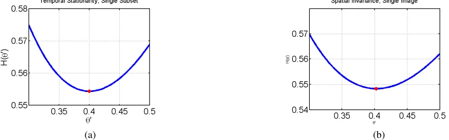
Fig. 1. True parameter isθ=.4. Minimizingθ0is indicated in red in each case. Plot of empirical cross entropy for (a) temporally stationary sequence on a single subset, and (b) spatially invariant parameter on multiple subsets.
V. EXAMPLE: HOMOGENEOUSISINGMODEL
We experimented with a (spatially) homogeneous Ising model, with edge parameter θij = .4 and node parameter
θi = 0on a200×200square grid of sites, where each interior
site is connected to its four nearest neighbors. The results are show in Figure 1. In (a), we consider a single subset U that is the middle row of the grid. The boundary ∂U consists of the row above and the row below. We generated a sequence of n= 198 configurations onGand computed
−1
n
n
X
i=1
logp(x(Ui)|x(∂Ui);θ0) (5)
for 161 evenly spaced θ0 values ranging from .3 to .5 (gran-ularity .00125). We found the minimizing θ0 to be the true parameter value of .4.
In (b), we consider a single configuration x on G, and let U1, . . . , Unbe then= 198rows ofGwith both an upper and
lower boundary row. We computed
1
n
n
X
i=1
logp(xUi|x∂Ui;θ
0) (6)
for the same 161θ0 values. In this case, the minimizingθ0 to be .4025.
VI. DISCUSSION
In this paper we have elaborated on the concept inherent in Maximum Pseudo-Likelihood, namely, that of using con-ditioning to simplify the task of parameter estimation, and have posed the problem as one of Minimum Conditional Description Length. The specific setting we have considered differs from the typical setting of MPL in that we have in mind temporal rather than spatial invariance, and we have here focused only on estimation of parameters within a single subset. Relaxing the spatial invariance assumption broadens the class of graphs and accompanying parameters to which we can apply this method. However, by requiring temporal stationarity we have imposed a new set of restrictions. More substantively, though, we feel that framing the problem as one of minimizing conditional description length is very
natural given that Markov/Gibbs fields are specified by their conditional distributions. This leads to the same MPL estimate when applied to a single configuration generated by a spatially invariant parameter, and as such, we feel that the Mini-mum Conditional Description Length perspective places the Maximum Pseudo-Likelihood estimate on a firmer theoretical footing.
As we mentioned in the Introduction, though this method can be applied to obtain estimatesθˆn
U1, . . . ,
ˆ
θn
Ukfor the
param-eters within different subsets, there is potential inconsistency of these estimates for nodes and edges contained within the intersection of these subsets. While resolving this, for example through alternating direction method of multipliers [5], remains to be done, we still believe there is value in the notion of taking a large intractable Markov random field and decomposing it into tractable conditional random fields, on which good parameter estimates can be obtained efficiently and in which exact inference and prediction can be performed with respect to these parameters, conditioned on the boundaries of these subsets. Indeed, it was shown in [21] that if the MRF is on an intractable graph, such that suboptimal inference and prediction will be performed with respect to whatever parameters are available, then there can be benefits to incorrectly estimating the parameters. In our case, good estimates would be obtained on each tractable conditional random field, and exact inference could be performed with respect to these parameters, but they may not yield a consistent estimate of the global parameter.
REFERENCES
[1] J. Besag, “Spatial Interaction and the Statistial Analysis of Lattice Systems,”J. of Roy. Stat. Soc. B, vol. 36, pp. 192-235, March 1974. [2] J. Besag, “Statistical Analysis of Non-lattice Data,”J. of Roy. Stat. Soc.
D, vol. 24, pp. 179-195, Sept. 1975.
[3] J. Besag, “Efficiency of pseudo-likelihood estimation for simple Gaussian fields,”Biometrika, Vol. 64, pp 616-618, 1977.
[4] S. Boyd and L. Vandenberghe,Convex Optimization, Cambridge Univer-sity Press, 2004.
[5] S. Boyd, N. Parikh, E. Chu, B. Peleato, and J. Eckstein, Distributed Optimization and Statistical Leaning via the Alternating Direction Method of Multipliers, Foundations in Trends in Machine Learning, Vol. 3, pp. 1-122, 2011.
[6] F. Comets, “On Consistency of a Class of Estimators for Exponential Families of Markov Random Fields on the Lattice,” The Annals of Statistics, Vol. 20, pp. 455-468, March 1992.
[7] T. Cover and J. Thomas,Elements of Information Theory, Wiley, 2005. [8] I. Csiszar and Z. Talata, “Consistent Estimation of the Basic
Neighbor-hood of Markov Random Fields,”The Annals of Statistics, Vol. 34, pp. 123-145, February 2006.
[9] S. Geman and D. Geman, “Stochastic Relaxation, Gibbs Distributions, and the Bayesian Restoration of Images,” IEEE Trans. PAMI, vol. 6, pp. 721–741, Nov. 1984.
[10] C. J. Geyer and E. A. Thompson, “Constrained Monte Carlo Maximum Likelihood for Dependent Data,”Journal of the Royal Statistical Society B, Vol. 54, 654-699, 1992.
[11] C. J. Geyer, “On the Convergence of Monte Carlo Maximum Likelihood Calculations,”Journal of the Royal Statistical Society B, Vol. 56, 261-274, 1994.
[12] B. Gidas, “Consistency of maximum likelihood and pseudolikelihood estimators for Gibbs distributions,”,Stochastic Differential Equations with Applications to Electronic/Computer Engineering, Control Theory, and Operations Research(W. Fleming and P. L. Lions, eds.), 1-17, Springer, Berlin.
[13] S. D. Pietra, V. D. Pietra, and J. Lafferty, “Inducing Features of Random Fields,” IEEE Trans. Pattern Analysis and Machine Intelligence, Vol. 19, No. 4, April 1997.
[14] M.G. Reyes and D.L. Neuhoff, Arithmetic Compression of Markov Random Fields, Seoul, Korea, ISIT 2009.
[15] M.G. Reyes and D.L. Neuhoff, Lossless Reduced Cutset Coding of Markov Random Fields, Snowbird, UT, DCC 2010.
[16] M.G. Reyes, Cutset Based Processing and Compression of Markov Random Fields, Ph.D. thesis, University of Michigan, April 2011. [17] M.G. Reyes and D.L. Neuhoff,Cutset Width and Spacing for Reduced
Cutset Coding of Markov Random Fields, submitted to ISIT 2016 (also in Deep Blue repository, University of Michigan).
[18] J. Rissanen, “Modeling by Shortest Data Description”,Automatica, Vol. 14, pp. 465-471, September 1978.
[19] S. Verdu and T. Weissman, “The Information Lost in Erasures”, IEEE Tran. Info. Thy., Vol. 54, No. 11, November 2008.
[20] M. J. Wainwright and M. I. Jordan, Graphical models, exponential families and variational inference, Berkeley Tech. Report 649, Sept. 2003. [21] M. J. Wainwright, “Estimating the ’Wrong’ Graphical Model: Benefits in the Computation Limited Setting”, Journal of Machine Learning Research, Vol. 7, pp. 1829-1859, September 2006.