R E S E A R C H
Open Access
A conjugate gradient algorithm for
large-scale unconstrained optimization
problems and nonlinear equations
Gonglin Yuan
1and Wujie Hu
1**Correspondence: [email protected] 1College of Mathematics and
Information Science, Guangxi University, Nanning, P.R. China
Abstract
For large-scale unconstrained optimization problems and nonlinear equations, we
propose a new three-term conjugate gradient algorithm under the Yuan–Wei–Lu line
search technique. It combines the steepest descent method with the famous
conjugate gradient algorithm, which utilizes both the relevant function trait and the
current point feature. It possesses the following properties: (i) the search direction has
a sufficient descent feature and a trust region trait, and (ii) the proposed algorithm
globally converges. Numerical results prove that the proposed algorithm is perfect
compared with other similar optimization algorithms.
MSC:
90C26
Keywords:
Conjugate gradient; Descent property; Global convergence
1 Introduction
It is well known that the model of small- and medium-scale smooth functions is simple
since it has many optimization algorithms, such as Newton, quasi-Newton, and bundle
algorithms. Note that three algorithms fail to effectively address large-scale optimization
problems because they need to store and calculate relevant matrices, whereas the
conju-gate gradient algorithm is successful because of its simplicity and efficiency.
The optimization model is an important mathematic problem since it has been applied
to various fields such as economics, engineering, and physics (see [1–12]). Fletcher and
Reeves [13] successfully address large-scale unconstrained optimization problems on the
basis of the conjugate gradient algorithm and obtained amazing achievements. The
con-jugate gradient algorithm is increasingly famous because of its simplicity and low
require-ment of calculation machine. In general, a good conjugate gradient algorithm
optimiza-tion algorithm includes a good conjugate gradient direcoptimiza-tion and an inexact line search
technique (see [14–18]). At present, the conjugate gradient algorithm is mostly applied to
smooth optimization problems, and thus, in this paper, we propose a modified LS
con-jugate gradient algorithm to solve large-scale nonlinear equations and smooth problems.
The common algorithms of addressing nonlinear equations include Newton and
quasi-Newton methods (see [19–21]), gradient-based, CG methods (see [22–24]), trust region
methods (see [25–27]), and derivative-free methods (see [28]), and all of them fail to
address large-scale problems. The famous optimization algorithms of spectral gradient
approach, limited-memory quasi-Newton method and conjugate gradient algorithm, are
suitable to solve large-scale problems. Li and Li [29] proposed various algorithms on the
basis of modified PRP conjugate gradient, which successfully solve large-scale nonlinear
equations.
A famous mathematic model is given by
min
f
(
x
)
|
x
∈
n,
(1.1)
where
f
:
n→
and
f
∈
C
2. The relevant model is widely used in life and production.
However, it is a complex mathematic model since it needs to meet various conditions in the
field [30–33]. Experts and scholars have conducted numerous in-depth studies and have
made some significant achievements (see [14, 34, 35]). It is well known that the steepest
descent algorithm is perfect since it is simple and its computational and memory
require-ments are low. It is regrettable that the steepest descent method sometimes fails to solve
problems due to the “sawtooth phenomenon”. To overcome this flaw, experts and scholars
presented an efficient conjugate gradient method, which provides high performance with
a simple form. In general, the mathematical formula for (1.1) is
x
k+1=
x
k+
α
kd
k,
k
∈ {
0, 1, 2, . . .
}
,
(1.2)
where
x
k+1is the next iteration point,
α
kis the step length, and
d
kis the search direction.
The famous weak Wolfe–Powell (WWP) line search technique is determined by
g
(
x
k+
α
kd
k)
Td
k≥
ρ
g
kTd
k(1.3)
and
f
(
x
k+
α
kd
k)
≤
f
k+
ϕα
kg
kTd
k,
(1.4)
where
ϕ
∈
(0, 1/2),
α
k> 0, and
ρ
∈
(
ϕ
, 1). The direction
d
k+1is often defined by the formula
d
k+1=
⎧
⎨
⎩
–
g
k+1+
β
kd
kif
k
≥
1,
–
g
k+1if
k
= 0,
(1.5)
where
β
k∈
. An increasing number of efficient conjugate gradient algorithms have been
proposed by different expressions of
β
kand
d
k(see [13, 36–42] etc.). The well-known PRP
algorithm is given by
β
kPRP=
g
T
k+1
(
g
k+1–
g
k)
g
kg
k,
(1.6)
the following creative formula (YWL) for the normal WWP line search technique and
obtained many fruitful theories:
f
(
x
k+
α
kd
k)
≤
f
(
x
k) +
ια
kg
kTd
k+
α
kmin
–
ι
1g
kTd
k,
ια
kd
k2/2
(1.7)
and
g
(
x
k+
α
kd
k)
Td
k≥
τ
g
kTd
k+
min
–
ι
1g
kTd
k,
ια
kd
k2,
(1.8)
where
ι
∈
(0,
12),
α
k> 0,
ι
1∈
(0,
ι
), and
τ
∈
(
ι
, 1). Further work can be found in [24]. Based on
the innovation of YWL line search technique, Yuan pay much attention to normal Armijo
line search technique and make further study. They proposed an efficient modified Armijo
line search technique:
f
(
x
k+
α
kd
k)
≤
f
(
x
k) +
λα
kg
kTd
k+
α
kmin
–
λ
1g
kTd
k,
λ
α
k2
d
k 2,
(1.9)
where
λ
,
γ
∈
(0, 1),
λ
1∈
(0,
λ
), and
α
kis the largest number of
{
γ
k|
k
= 0, 1, 2, . . .
}
. In
addi-tion, experts and scholars pay much attention to the three-term conjugate gradient
for-mula. Zhang et al. [44] proposed the famous formula
d
k+1= –
g
k+1+
g
Tk+1
y
kd
k–
d
Tkg
k+1y
kg
kTg
k.
(1.10)
Nazareth [45] proposed the new formula
d
k+1= –
y
k+
y
T ky
ky
T kd
kd
k+
y
T k–1y
ky
T k–1d
k–1d
k–1,
(1.11)
where
y
k=
g
k+1–
g
kand
s
k=
x
k+1–
x
k. These two conjugate gradient methods have a
suffi-cient descent property but fail to have the trust region feature. To improve these methods,
Yuan et al. [46, 47] make a further study and get some good results. This inspires us to
continue the study and extend the conjugate gradient methods to get better results. In
this paper, motivated by in-depth discussions, we express a modified conjugate gradient
algorithm, which has the following properties:
•
The search direction has a sufficient descent feature and a trust region trait.
•
Under mild assumptions, the proposed algorithm possesses the global convergence.
•
The new algorithm combines the steepest descent method with the conjugate
gradient algorithm.
•
Numerical results prove that it is perfect compared to other similar algorithms.
The rest of the paper is organized as follows. The next section presents the necessary
properties of the proposed algorithm. The global convergence is stated in Sect. 3. In Sect. 4,
we report the corresponding numerical results. In Sect. 5, we introduce the large-scale
nonlinear equations and express the new algorithm. Some necessary properties are listed
in Sect. 6. The numerical results are reported in Sect. 7. Without loss of generality,
f
(
x
k)
Algorithm 2.1
Modified three-term conjugate gradient algorithm for optimization model
Step 1: (Initiation) Choose an initial point
x
0,
ι
∈
(0,
12)
,
ι
1∈
(0,
ι
)
,
η
i> 0
(
i
= 1, 2, 3, 4, 5
),
τ
∈
(
ι
, 1)
, and positive constants
ε
∈
(0, 1)
. Let
k
= 0
and
d
0= –
g
0.
Step 2: Stop if
g
k≤
ε
.
Step 3: Find the step length
α
ksimilar to (1.7) and (1.8).
Step 4: Set a new iteration point of
x
k+1=
x
k+
α
kd
k.
Step 5: Update the search direction by (2.1).
Step 6: If
g
k+1≤
ε
, then stop. Otherwise, go to the next step.
Step 7: Let
k
:=
k
+ 1
, and return to Step 3.
2 New modified conjugate gradient algorithm
Experts and scholars have conducted thorough research on the conjugate gradient
algo-rithm and have obtained rich theoretical achievements. In light of the previous work by
experts on the conjugate gradient algorithm, a sufficient descent feature is necessary for
the global convergence. Thus, we express a new conjugate gradient algorithm under the
YWL line search technique as follows:
d
k+1=
⎧
⎨
⎩
–
η
1g
k+1+ (1 –
η
1)(
d
kTg
k+1y
∗k–
g
kT+1y
k∗d
k)/
δ
if
k
≥
1,
–
g
k+1if
k
= 0,
(2.1)
where
δ
=
max(min(
η
5|
s
Tky
∗k|
,
|
d
Tky
∗k|
),
η
2y
∗kd
k,
η
3g
k2) +
η
4∗
d
k2,
y
∗k=
g
k+1–
gk+1 2gk2
g
k,
and
η
i> 0 (
i
= 1, 2, 3, 4, 5). The search direction is well defined, and its properties are stated
in the next section. Now, we introduce a new conjugate gradient algorithm called
Algo-rithm 2.1.
3 Important characteristics
This section lists some important properties of sufficient descent, the trust region, and
the global convergence of Algorithm 2.1. It expresses the necessary proof.
Lemma 3.1
If search direction d
kmeets condition of
(2.1),
then
g
kTd
k= –
η
1g
k2(3.1)
and
d
k≤
η
1+ 2(1 –
η
1)/
η
2g
k.
(3.2)
Proof
It is obvious that formulas of (3.1) and (3.2) are true for
k
= 0.
Now consider the condition
k
≥
1. Similarly to (2.1), we have
g
kT+1d
k+1=
g
kT+1–
η
1g
k+1+ (1 –
η
1)
d
kTg
k+1y
∗k–
g
kT+1y
∗kd
k/
δ
= –
η
1g
k+12+ (1 –
η
1)
g
kT+1d
kTg
k+1y
∗k–
g
kT+1g
kT+1y
∗kd
k/
δ
and
d
k+1=
–
η
1g
k+1+ (1 –
η
1)
d
Tkg
k+1y
∗k–
g
kT+1y
∗kd
k/
δ
≤
η
1g
k+1+ 2(1 –
η
1)
g
k+1y
∗kd
k/
δ
≤
η
1g
k+1+ 2(1 –
η
1)
g
k+1y
∗kd
k/
η
2y
∗kd
k=
η
1+ 2(1 –
η
1)/
η
2g
k+1.
Thus, the statement is proved.
Similarly to (3.1) and (3.2), the algorithm has a sufficient descent feature and a trust
region trait. To obtain the global convergence, we propose the following necessary
as-sumptions.
Assumption 1
(i) The level set of
π
=
{
x
|
f
(
x
)
≤
f
(
x
0)
}
is bounded.
(ii) The objective function
f
∈
C
2is bounded from below, and its gradient function
g
is
Lipschitz continuous, thats is, there exists a constant
ζ
such that
g
(
x
) –
g
(
y
)
≤
ζ
x
–
y
,
x
,
y
∈
R
n.
(3.3)
The existence and necessity of the step length
α
kare established in [43]. In view of
the discussion and established technique, the global convergence of the proposed
algorithm is expressed as follows.
Theorem 3.1
If Assumptions
(i)–(ii)
are satisfied and the relative sequences of
{
x
k}
,
{
d
k}
,
{
g
k}
,
and
{
α
k}
are generated by Algorithm
2.1,
then
lim
k→∞
g
k= 0.
(3.4)
Proof
By (1.7), (3.1), and (3.3) we have
f
(
x
k+
α
kd
k)
≤
f
k+
ια
kg
Tkd
k+
α
kmin
–
ι
1g
kTd
k,
ια
kd
k2/2
≤
f
k+
ια
kg
Tkd
k–
α
kι
1g
kTd
k≤
f
k+
α
k(
ι
–
ι
1)
g
kTd
k≤
f
k–
η
1α
k(
ι
–
ι
1)
g
k2.
Summing these inequalities from
k
= 0 to
∞
, under Assumption (ii), we obtain
∞
k=0
η
1α
k(
ι
–
ι
1)
g
k2≤
f
(
x
0) –
f
∞< +
∞
.
(3.5)
This means that
lim
k→∞
α
kg
kSimilarly to (1.8) and (3.1), we obtain
g
(
x
k+
α
kd
k)
Td
k≥
τ
g
kTd
k+
min
–
ι
1g
kTd
k,
ια
kd
k2≥
τ
g
kTd
k.
Thus, we obtain the following inequality:
–
η
1(
τ
– 1)
g
k2≤
(
τ
– 1)
g
kTd
k≤
g
(
x
k+
α
kd
k) –
g
(
x
k)
Td
k≤
g
(
x
k+
α
kd
k) –
g
(
x
k)
d
k≤
α
kζ
d
k2,
where the last inequality is obtained since the gradient function is Lipschitz continuous.
Then, we have
α
k≥
(1 –
τ
)
η
1g
k2ζ
d
k2≥
(1 –
τ
)
η
1g
k2(
ζ
(
η
1+ 2(1 –
η
1)/
η
2)
2g
k2))
=
(1 –
τ
)
η
1(
ζ
(
η
1+ 2(1 –
η
1)/
η
2)
2)
.
By (3.6) we arrive at the conclusion
lim
k→∞
g
k2
= 0,
as claimed.
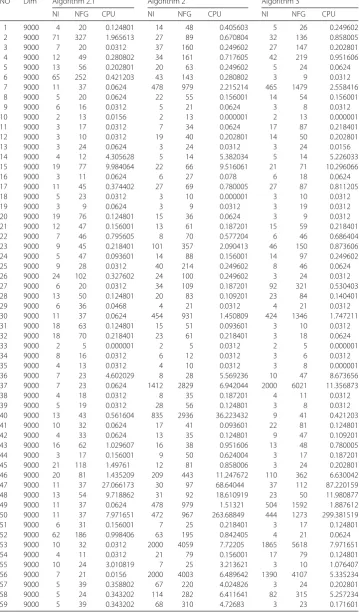
4 Numerical results
In this section, we list the numerical result in terms of the algorithm characteristics NI,
NFG, and CPU, where NI is the total iteration number, NFG is the sum of the calculation
frequency of the objective function and gradient function, and CPU is the calculation time
in seconds.
4.1 Problems and test experiments
The tested problems listed in Table 1 stem from [48]. At the same time, we introduce
two different algorithms into this section to measure the objective algorithm efficiency
through the tested problems. We denote the two algorithms as Algorithm 2 and
Algo-rithm 3. They are different from AlgoAlgo-rithm 2.1 only at Step 5. One is determined by (1.10),
and the other is computed by (1.11).
Stopping rule:
If the inequality
|
f
(
x
k)
|
>
e
1is correct, let
stop
1 =
|f(xk|)–f(xf(xk+1)|k)|
or
stop
1 =
|
f
(
x
k) –
f
(
x
k+1)
|
. The algorithm stops when one of the following conditions is satisfied:
g
(
x
)
<
, the iteration number is greater than 2000, or
stop
1 <
e
2, where
e
1=
e
2= 10
–5and
= 10
–6. In Table 1, “No” and “problem” represent the index of the the tested problems
and the name of the problem, respectively.
Initiation:
ι
= 0.3,
ι
1= 0.1,
τ
= 0.65,
η
1= 0.65,
η
2= 0.001,
η
3= 0.001,
η
4= 0.001,
η
5= 0.1.
Dimension:
1200, 3000, 6000, 9000.
Table 1
Test problems
No. Problem
1 Extended Freudenstein and Roth Function 2 Extended Trigonometric Function 3 Extended Rosenbrock Function 4 Extended White and Holst Function 5 Extended Beale Function 6 Extended Penalty Function 7 Perturbed Quadratic Function 8 Raydan 1 Function
9 Raydan 2 Function 10 Diagonal 1 Function 11 Diagonal 2 Function 12 Diagonal 3 Function 13 Hager Function
14 Generalized Tridiagonal 1 Function 15 Extended Tridiagonal 1 Function
16 Extended Three Exponential Terms Function 17 Generalized Tridiagonal 2 Function 18 Diagonal 4 Function
19 Diagonal 5 Function
20 Extended Himmelblau Function 21 Generalized PSC1 Function 22 Extended PSC1 Function 23 Extended Powell Function
24 Extended Block Diagonal BD1 Function 25 Extended Maratos Function
26 Extended Cliff Function
27 Quadratic Diagonal Perturbed Function 28 Extended Wood Function
29 Extended Hiebert Function 30 Quadratic Function QF1 Function 31 Extended Quadratic Penalty QP1 Function 32 Extended Quadratic Penalty QP2 Function 33 A Quadratic Function QF2 Function 34 Extended EP1 Function
35 Extended Tridiagonal-2 Function 36 BDQRTIC Function (CUTE) 37 TRIDIA Function (CUTE)
No. Problem
38 ARWHEAD Function (CUTE) 38 ARWHEAD Function (CUTE) 40 NONDQUAR Function (CUTE) 41 DQDRTIC Function (CUTE) 42 EG2 Function (CUTE) 43 DIXMAANA Function (CUTE) 44 DIXMAANB Function (CUTE) 45 DIXMAANC Function (CUTE) 46 DIXMAANE Function (CUTE) 47 Partial Perturbed Quadratic Function 48 Broyden Tridiagonal Function 49 Almost Perturbed Quadratic Function 50 Tridiagonal Perturbed Quadratic Function 51 EDENSCH Function (CUTE)
52 VARDIM Function (CUTE) 53 STAIRCASE S1 Function 54 LIARWHD Function (CUTE) 55 DIAGONAL 6 Function 56 DIXON3DQ Function (CUTE) 57 DIXMAANF Function (CUTE) 58 DIXMAANG Function (CUTE) 59 DIXMAANH Function (CUTE) 60 DIXMAANI Function (CUTE) 61 DIXMAANJ Function (CUTE) 62 DIXMAANK Function (CUTE) 63 DIXMAANL Function (CUTE) 64 DIXMAAND Function (CUTE) 65 ENGVAL1 Function (CUTE) 66 FLETCHCR Function (CUTE) 67 COSINE Function (CUTE)
68 Extended DENSCHNB Function (CUTE) 69 DENSCHNF Function (CUTE) 70 SINQUAD Function (CUTE) 71 BIGGSB1 Function (CUTE)
72 Partial Perturbed Quadratic PPQ2 Function 73 Scaled Quadratic SQ1 Function
A list of the numerical results with the corresponding problem index is listed in Table 2.
Then, based on the technique in [49], the plots of the corresponding figures are presented
for the three discussed algorithms.
Other case:
To save the paper space, we only list the data of dimension of 9000, and the
remaining data are listed in the attachment.
4.2 Results and discussion
Table 2
Numerical results
NO Dim Algorithm 2.1 Algorithm 2 Algorithm 3
NI NFG CPU NI NFG CPU NI NFG CPU
1 9000 4 20 0.124801 14 48 0.405603 5 26 0.249602
2 9000 71 327 1.965613 27 89 0.670804 32 136 0.858005
3 9000 7 20 0.0312 37 160 0.249602 27 147 0.202801
4 9000 12 49 0.280802 34 161 0.717605 42 219 0.951606
5 9000 13 56 0.202801 20 63 0.249602 5 24 0.0624
6 9000 65 252 0.421203 43 143 0.280802 3 9 0.0312
7 9000 11 37 0.0624 478 979 2.215214 465 1479 2.558416
8 9000 5 20 0.0624 22 55 0.156001 14 54 0.156001
9 9000 6 16 0.0312 5 21 0.0624 3 8 0.0312
10 9000 2 13 0.0156 2 13 0.000001 2 13 0.000001
11 9000 3 17 0.0312 7 34 0.0624 17 87 0.218401
12 9000 3 10 0.0312 19 40 0.202801 14 50 0.202801
13 9000 3 24 0.0624 3 24 0.0312 3 24 0.0156
14 9000 4 12 4.305628 5 14 5.382034 5 14 5.226033
15 9000 19 77 9.984064 22 66 9.516061 21 71 10.296066
16 9000 3 11 0.0624 6 27 0.078 6 18 0.0624
17 9000 11 45 0.374402 27 69 0.780005 27 87 0.811205
18 9000 5 23 0.0312 3 10 0.000001 3 10 0.0312
19 9000 3 9 0.0624 3 9 0.0312 3 19 0.0312
20 9000 19 76 0.124801 15 36 0.0624 3 9 0.0312
21 9000 12 47 0.156001 13 61 0.187201 15 59 0.218401
22 9000 7 46 0.795605 8 70 0.577204 6 46 0.686404
23 9000 9 45 0.218401 101 357 2.090413 46 150 0.873606
24 9000 5 47 0.093601 14 88 0.156001 14 97 0.249602
25 9000 9 28 0.0312 40 214 0.249602 8 46 0.0624
26 9000 24 102 0.327602 24 100 0.249602 3 24 0.0312
27 9000 6 20 0.0312 34 109 0.187201 92 321 0.530403
28 9000 13 50 0.124801 20 83 0.109201 23 84 0.140401
29 9000 6 36 0.0468 4 21 0.0312 4 21 0.0312
30 9000 11 37 0.0624 454 931 1.450809 424 1346 1.747211
31 9000 18 63 0.124801 15 51 0.093601 3 10 0.0312
32 9000 18 70 0.218401 23 61 0.218401 3 18 0.0624
33 9000 2 5 0.000001 2 5 0.0312 2 5 0.000001
34 9000 8 16 0.0312 6 12 0.0312 3 6 0.0312
35 9000 4 13 0.0312 4 10 0.0312 3 8 0.000001
36 9000 7 23 4.602029 8 28 5.569236 10 47 8.673656
37 9000 7 23 0.0624 1412 2829 6.942044 2000 6021 11.356873
38 9000 4 18 0.0312 8 35 0.187201 4 11 0.0312
39 9000 5 19 0.0312 28 56 0.124801 3 8 0.0312
40 9000 13 43 0.561604 835 2936 36.223432 9 41 0.421203
41 9000 10 32 0.0624 17 41 0.093601 22 81 0.124801
42 9000 4 33 0.0624 13 35 0.124801 9 47 0.109201
43 9000 16 62 1.029607 16 38 0.951606 13 48 0.780005
44 9000 3 17 0.156001 9 50 0.624004 3 17 0.187201
45 9000 21 118 1.49761 12 81 0.858006 3 24 0.202801
46 9000 20 81 1.435209 209 443 11.247672 110 362 6.630042
47 9000 11 37 27.066173 30 97 68.64044 37 112 87.220159
48 9000 13 54 9.718862 31 92 18.610919 23 50 11.980877
49 9000 11 37 0.0624 478 979 1.51321 504 1592 1.887612
50 9000 11 37 7.971651 472 967 263.68849 444 1273 299.381519
51 9000 6 31 0.156001 7 25 0.218401 3 17 0.124801
52 9000 62 186 0.998406 63 195 0.842405 4 21 0.0624
53 9000 10 32 0.0312 2000 4059 7.72205 1865 5618 7.971651
54 9000 4 11 0.0312 21 79 0.156001 17 79 0.124801
55 9000 10 24 3.010819 7 25 3.213621 3 10 1.076407
56 9000 7 21 0.0156 2000 4003 6.489642 1390 4107 5.335234
57 9000 5 39 0.358802 67 220 4.024826 3 24 0.202801
58 9000 5 24 0.343202 114 282 6.411641 82 315 5.257234
Table 2
(
Continued
)
NO Dim Algorithm 2.1 Algorithm 2 Algorithm 3
NI NFG CPU NI NFG CPU NI NFG CPU
60 9000 18 74 1.294808 206 437 11.107271 119 363 6.957645
61 9000 5 39 0.358802 85 247 4.929632 3 24 0.218401
62 9000 4 32 0.234001 4 32 0.249602 3 22 0.187201
63 9000 3 22 0.187201 3 22 0.187201 3 22 0.187201
64 9000 5 39 0.343202 23 147 1.747211 3 23 0.218401
65 9000 12 59 15.334898 14 51 14.944896 7 21 6.130839
66 9000 3 9 1.62241 2000 4022 1114.767546 529 2196 443.526443
67 9000 5 28 0.093601 15 58 0.280802 3 23 0.0312
68 9000 13 55 0.109201 11 27 0.0624 9 25 0.0624
69 9000 16 73 0.218401 24 55 0.187201 20 70 0.171601
70 9000 4 13 2.542816 41 203 36.332633 35 231 37.783442
71 9000 11 35 0.093601 2000 4014 6.708043 1491 4631 5.600436
72 9000 9 30 21.85574 1089 3897 2675.588751 287 1015 704.391315
[image:9.595.117.478.96.263.2]73 9000 19 65 0.093601 607 1269 1.856412 669 2062 2.293215
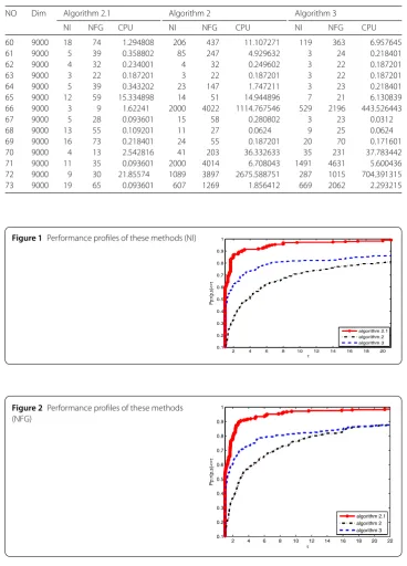
Figure 1Performance profiles of these methods (NI)
Figure 2Performance profiles of these methods (NFG)
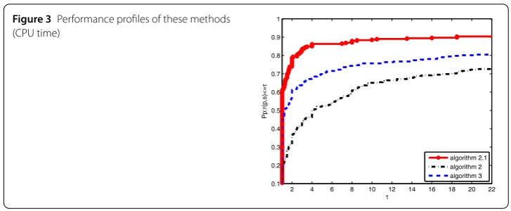
objective algorithm successfully fully utilizes its outstanding characteristics. Therefore, it
saves time compared to the other algorithms in addressing complex problems.
5 Nonlinear equations
The model of nonlinear equations is given by
Figure 3Performance profiles of these methods (CPU time)
where the function of
h
is continuously differentiable and monotonous, and
x
∈
R
n, that
is,
h
(
x
) –
h
(
y
)
(
x
–
y
) > 0,
∀
x
,
y
∈
R
n.
Scholars and writers paid much attention to this model since it significantly influences
various fields such as physics and computer technology (see [1–3, 8–11]), and it has
re-sulted in many fruitful theories and good techniques (see [47, 50–54]). By mathematical
calculations we obtain that (5.1) is equivalent to the model
min
F
(
x
),
(5.2)
where
F
(
x
) =
h(x2)2, and
·
is the Euclidean norm. Then, we pay much attention to
the mathematical model (5.2) since (5.1) and (5.2) have the same solution. In general, the
mathematical formula for (5.2) is
x
k+1=
x
k+
α
kd
k. Now, we introduce the following famous
line search technique into this paper [47, 55]:
–
h
(
x
k+
α
kd
k)
Td
k≥
σ α
kh
(
x
k+
α
kd
k)
d
k2,
(5.3)
where
α
k=
max
{
s
,
s
ρ
,
s
ρ
2, . . .
}
,
s
,
ρ
> 0,
ρ
∈
(0, 1), and
σ
> 0. Solodov [56] proposes a
projec-tion proximal point algorithm in a Hilbert space that finds the zeros of set-valued maximal
monotone operators. Ceng and Yao [57–60] paid much attention to the research in Hilbert
spaces and obtained successful achievements. Solodov and Svaiter [61] applied the
projec-tion technique to large-scale nonlinear equaprojec-tions and obtained some ideal achievements.
For the projection-based technique, the famous formula
h
(
w
k)
T(
x
k–
w
k) > 0
is flexible, where
w
k=
x
k+
α
kd
k. The search direction is extremely important for the
pro-posed algorithm since it largely determines the efficiency. Likewise, the algorithm contains
the perfect line search technique. By the monotonicity of
h
(
x
) we obtain
h
(
w
k)
Tx
∗–
w
kAlgorithm 5.1
Modified three-term conjugate gradient algorithm for large-scale
nonlin-ear equations
Step 1: Choose an initial point
x
1∈
R
n,
σ
> 0
,
s
> 0
,
ρ
∈
(0, 1)
,
η
i> 0
(
i
= 1, 2, 3, 4, 5
), and
positive constants
ε
∈
(0, 1)
. Let
k
= 1
.
Step 2: Stop if
h
(
x
k)
≤
ε
. Otherwise, calculate
d
k+1similar to (5.6).
Step 3: Find the step length
α
ksimilar to (5.3).
Step 4: Reset the new iteration point of
w
k=
x
k+
α
kd
k.
Step 5: If
h
(
w
k)
≤
ε
, then stop and set
x
k+1=
w
k. Otherwise, calculate
x
k+1similar to
(5.5).
Step 6: Let
k
:=
k
+ 1
and return to Step 2.
where
x
∗is the solution of
h
(
x
∗) = 0. We consider the hyperplane
=
x
∈
R
n|
h
(
w
k)
T(
x
–
w
k) = 0
.
(5.4)
It is obvious that the hyperplane separates the current iteration point of
x
kfrom the zeros
of the mathematical model (5.1). Then, we need to calculate the next iteration point
x
k+1through projection of current point
x
k. Therefore, we give the following formula for the
next point:
x
k+1=
x
k–
h
(
w
k)
T(
x
k–
w
k)
h
(
w
k)
h
(
w
k)
2.
(5.5)
In [55], it is proved that formula (5.5) is effective since it not only obtains perfect numerical
results but also has perfect theoretical characteristics. Thus, we introduce it here. The
formula of the search direction
d
k+1is given by
d
k+1=
⎧
⎨
⎩
–
η
1h
k+1+ (1 –
η
1)(
d
Tkh
k+1y
∗k–
h
Tk+1y
k∗d
k)/
δ
if
k
≥
1,
–
h
k+1if
k
= 0,
(5.6)
where
δ
=
max(min(
η
5|
s
Tky
∗k|
,
|
d
Tky
∗k|
),
η
2y
∗kd
k,
η
3g
k2)+
η
4∗
d
k2,
y
∗k=
h
k+1–
hk+1 2hk2
h
k,
and
η
i> 0 (
i
= 1, 2, 3). Now, we express the specific content of the proposed algorithm.
6 The global convergence of Algorithm 5.1
First, we make the following necessary assumptions.
Assumption 2
(i) The objective model of (5.1) has a nonempty solution set.
(ii) The function
h
is Lipschitz continuous on
R
n, which means that there is a positive
constant
L
such that
h
(
x
) –
h
(
y
)
≤
L
x
–
y
,
∀
x
,
y
∈
R
n.
(6.1)
By Assumption 2(ii) it is obvious that
where
θ
is a positive constant. Then, the necessary properties of the search direction are
the following (we omit the proof ):
h
Tkd
k= –
η
1h
kh
k(6.3)
and
d
k≤
η
1+ 2(1 –
η
1)/
η
2h
k.
(6.4)
Now, we give some lemmas, which we utilize to obtain the global convergence of the
pro-posed algorithm.
Lemma 6.1
If Assumption
2
holds
,
the relevant sequence
{
x
k}
is produced by Algorithm
5.1,
and the point x
∗is the solution of the objective model
(5.1).
We obtain that the formula
x
k+1–
x
∗ 2≤
x
k–
x
∗2
–
x
k+1–
x
k2is correct and the sequence
{
x
k}
is bounded
.
Furthermore
,
either the last iteration point is
the solution of the objective model and the sequence of
{
x
k}
is bounded
,
or the sequence of
{
x
k}
is infinite and satisfies the condition
∞
k=0
x
k+1–
x
k2<
∞
.
This paper merely proposes, but omits, the relevant proof since it is similar to the proof
in [61].
Lemma 6.2
Algorithm
5.1
generates an iteration point in a finite number of iteration steps
,
which satisfies the formula of x
k+1=
x
k+
α
kd
kif Assumption
2
holds
.
Proof
We denote
=
N
∪ {
0
}
. We suppose that Algorithm 5.1 has terminated or the
for-mula
h
k→
0 is erroneous. This means that there exists a constant
ε
∗such that
h
k≥
ε
∗,
k
∈
.
(6.5)
We prove this conclusion by contradiction. Suppose that certain iteration indexes
k
∗fail
to meet the condition (5.3) of the line search technique. Without loss of generality, we
denote the corresponding step length as
α
k(l∗), where
α
k(l∗)=
ρ
ls
. This means that
–
h
x
k∗+
α
k(l∗)d
k∗ Td
k∗<
σ α
k(l∗)h
x
k∗+
α
k(l∗)d
k∗d
k∗2.
By (6.3) and Assumption 2(ii) we obtain
h
k∗2= –
η
1h
Tk∗d
k∗=
η
1h
x
k∗+
α
(kl∗)d
k∗–
h
(
x
k∗)
Td
k∗–
h
x
k∗+
α
k(l∗)d
k∗ Td
k∗<
η
1By (6.3) and (6.4) we have
h
x
k∗+
α
(kl∗)d
k∗≤
h
x
k∗+
α
k(l∗)d
k∗–
h
(
x
k∗)
+
h
(
x
k∗)
≤
L
α
(kl∗)d
k∗+
θ
≤
Ls
θ
η
1+ 2(1 –
η
1)/
η
2+
θ
.
By (6.6) we obtain
α
(kl∗)>
h
k ∗2η
1[
L
+
σ
h
(
x
k∗+
α
k(l∗)d
k∗)
]
d
k∗2>
h
k∗2
η
1[
L
+
σ
(
Ls
θ
(
η
1+ 2(1 –
η
1)/
η
2) +
θ
)]
d
k∗2>
η
2 2
η
1[
L
+
σ
(
Ls
θ
(
η
1+ 2/
η
3) +
θ
)](2(1 –
η
1) +
η
2η
1)
2,
∀
l
∈
.
It is obvious that this formula fails to meet the definition of the step length
α
k(l∗). Thus,
we conclude that the proposed line search technique is reasonable and necessary. In other
words, the line search technique generates a positive constant
α
kin a finite frequency of
backtracking repetitions. By the established conclusion we propose the following theorem
on the global convergence of the proposed algorithm.
Theorem 6.1
If Assumption
2
holds and the relevant sequences
{
d
k,
α
k,
x
k+1,
h
k+1}
are
cal-culated using Algorithm
5.1,
then
lim inf
k→∞
h
k= 0.
(6.6)
Proof
We prove this by contradiction. This means that there exist a constant
ε
0> 0 and
an index
k
0such that
h
k≥
ε
0,
∀
k
≥
k
0.
On the one hand, by (6.2) and (6.4) we obtain
d
k≤
η
1+ 2(1 –
η
1)/
η
2h
k≤
η
1+ 2(1 –
η
1)/
η
2θ
,
∀
k
∈
.
(6.7)
On the other hand, from (6.3) we have
d
k≥
η
1h
k≥
η
1θ
.
(6.8)
These inequalities indicate that the sequence of
{
d
k}
is bounded. This means that there
exist an accumulation point
d
∗and the corresponding infinite set
N
1such that
lim
k→∞
d
k=
d
∗
,
k
∈
N
By Lemma 6.1 we obtain that the sequence of
{
x
k}
is bounded. Thus, there exist an infinite
index set
N
2⊂
N
1and an accumulation point
x
∗that meet the formula
lim
k→∞
x
k=
x
∗
,
∀
k
∈
N
2
.
By Lemmas 6.1 and 6.2 we obtain
α
kd
k→
0,
k
→ ∞
.
Since
{
d
k}
is bounded, we obtain
lim
k→∞
α
k= 0.
(6.9)
By the definition of
α
kwe obtain the following inequality:
–
h
x
k+
α
∗kd
k Td
k≤
σ α
∗kh
x
k+
α
∗kd
kd
k2,
(6.10)
where
α
∗k=
α
k/
ρ
. Now, we take the limit on both sides of (6.10) and (6.3) and obtain
h
x
∗Td
∗> 0
and
h
x
∗Td
∗≤
0.
The obtained contradiction completes the proof.
7 The results of nonlinear equations
In this section, we list the relevant numerical results of nonlinear equations and present
the objective function
h
(
x
) = (
f
1(
x
),
f
2(
x
), . . . ,
f
n(
x
)), where the relevant functions’
informa-tion is listed in Table 1.
7.1 Problems and test experiments
To measure the efficiency of the proposed algorithm, in this section, we compare this
method with (1.10) (as Algorithm 6) using three characteristics “NI”, “NG”, and “CPU”
and the remind that Algorithm 6 is identical to Algorithm 5.1. “NI” presents the number
of iterations, “NG” is the calculation frequency of the function, and “CPU” is the time of
the process in addressing the tested problems. In Table 1, “No” and “problem” express the
indices and the names of the test problems.
Stopping rule:
If
g
k≤
ε
or the whole iteration number is greater than 2000, the
algo-rithm stops.
Initiation:
ε
= 1
e
–5,
σ
= 0.8,
s
= 1,
ρ
= 0.9,
η
1= 0.85,
η
2=
η
3= 0.001,
η
4=
η
5= 0.1.
Dimension:
3000, 6000, 9000.
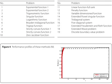
Table 3
Test problems
No. Problem
1 Exponential function 1
2 Exponential function 2
3 Trigonometric function
4 Singular function
5 Logarithmic function
6 Broyden tridiagonal function
7 Trigexp function
8 Strictly convex function 1
9 Strictly convex function 2
10 Zero Jacobian function
No. Problem
11 Linear function-full rank 12 Penalty function
13 Variable dimensioned function 14 Extended Powel singular function 15 Tridiagonal system
16 Five-diagonal system
17 Extended Freudentein and Roth function 18 Extended Wood problem
[image:15.595.117.478.94.364.2]19 Discrete boundary value problem
Figure 4Performance profiles of these methods (NI)
The numerical results with the corresponding problem index are listed in Table 4. Then,
by the technique in [49], the plots of the corresponding figures are presented for two
dis-cussed algorithms.
7.2 Results and discussion
From the above figures, we safely arrive at the conclusion that the proposed algorithm is
perfect compared to similar optimization methods since the algorithm (1.10) is perfect to
a large extent. In Fig. 4 we see that the proposed algorithm quickly arrives at a value of 1.0,
whereas the left one slowly approaches 1.0. This means that the objective method is
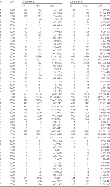
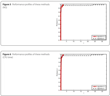
suc-cessful and efficient for addressing complex problems in our life and work. It is well known
that the calculation time is one of the most essential characteristics in an evaluation index
of the efficiency of an algorithm. From Figs. 5 and 6, it is obvious that the two algorithms
are good since their corresponding point values arrive at 1.0. This result expresses that the
above two algorithms solve all of the tested problems and that the proposed algorithm is
efficient.
8 Conclusion
This paper focuses on the three-term conjugate gradient algorithms and use them to solve
the optimization problems and the nonlinear equations. The given method has some good
properties.
Table 4
Numerical results
NO Dim Algorithm 5.1 Algorithm 6
NI NFG CPU NI NFG CPU
1 3000 161 162 3.931225 146 147 4.149627
1 6000 126 127 12.760882 115 116 11.122871
1 9000 111 112 22.464144 99 100 19.515725
2 3000 5 76 1.185608 5 76 1.060807
2 6000 6 91 4.758031 5 76 4.009226
2 9000 5 62 6.926444 5 62 6.754843
3 3000 33 228 3.276021 18 106 1.778411
3 6000 40 275 15.490899 18 106 6.084039
3 9000 40 285 33.243813 18 106 12.54248
4 3000 4 61 0.842405 4 61 0.936006
4 6000 4 47 2.698817 4 61 3.322821
4 9000 4 47 5.226033 4 61 6.817244
5 3000 23 237 3.244821 23 237 3.354022
5 6000 25 263 14.133691 25 263 13.930889
5 9000 26 278 30.186193 26 278 30.092593
6 3000 1999 29986 382.951255 1999 29986 365.369942
6 6000 88 1307 68.141237 1999 29986 1484.240314
6 9000 65 962 101.806253 1999 29986 3113.998361
7 3000 4 47 0.748805 3 46 0.624004
7 6000 4 47 2.589617 3 46 2.386815
7 9000 4 47 5.257234 3 46 5.054432
8 3000 25 156 2.854818 17 142 1.872012
8 6000 32 189 10.826469 18 162 8.377254
8 9000 28 192 21.512538 19 174 18.938521
9 3000 10 151 1.934412 5 76 1.014007
9 6000 4 61 3.510023 5 76 3.884425
9 9000 4 61 6.614442 6 91 9.609662
10 3000 1999 29986 386.804479 1999 29986 359.816306
10 6000 1999 29986 1523.068963 1999 29986 1469.59182
10 9000 1999 29986 3164.339884 1999 29986 3087.712193
11 3000 498 7457 98.32743 499 7472 93.101397
11 6000 498 7457 385.026068 499 7472 367.787958
11 9000 498 7457 794.07629 498 7457 774.825767
12 3000 1999 2000 51.059127 1999 2000 46.238696
12 6000 1999 2000 199.322478 1999 2000 185.71919
12 9000 1999 2000 405.680601 1999 2000 391.234908
13 3000 1 2 0.0312 1 2 0.0624
13 6000 1 2 0.156001 1 2 0.187201
13 9000 1 2 0.140401 1 2 0.249602
14 3000 1999 29972 400.220565 1999 29973 362.671125
14 6000 1999 29972 1544.316299 1999 29973 1460.294161
14 9000 1999 29972 3197.287295 1999 29973 3105.168705
15 3000 4 61 0.733205 4 61 0.733205
15 6000 4 61 3.790824 4 61 3.026419
15 9000 4 61 6.552042 4 61 6.146439
16 3000 5 62 1.060807 5 62 0.858006
16 6000 5 62 3.400822 5 62 3.291621
16 9000 5 62 6.942044 5 62 6.25564
17 3000 6 77 1.326009 6 91 1.216808
17 6000 6 77 4.243227 6 91 4.570829
17 9000 6 77 8.548855 6 91 9.40686
18 3000 5 76 0.936006 5 76 0.920406
18 6000 5 76 3.900025 5 76 3.775224
18 9000 5 76 8.533255 5 76 7.86245
19 3000 108 1060 15.5689 141 1272 17.565713
19 6000 81 788 44.429085 114 1029 53.820345
Figure 5Performance profiles of these methods (NG)
Figure 6Performance profiles of these methods (CPU time)
(ii) The given algorithm can be used for not only the normal unstrained optimization
problems but also for the nonlinear equations. Both algorithms for these two
problems have the global convergence under general conditions.
(iii) Large-scale problems are done by the given problems, which shows that the new
algorithms are very effective.
Acknowledgements
The authors would like to thank the editor and the referees for their interesting comments, which greatly improved our paper. This work is supported by the National Natural Science Foundation of China (Grant No. 11661009), the Guangxi Science Fund for Distinguished Young Scholars (No. 2015GXNSFGA139001), and the Guangxi Natural Science Key Fund (No. 2017GXNSFDA198046). Innovation Project of Guangxi Graduate Education (No. YCSW2018046)
Competing interests
The authors declare to have no competing interests.
Authors’ contributions
The work of Dr. GY is organizing and checking this paper, and Dr. WH mainly has done the experiments of the algorithms and written the codes. All authors read and approved the final manuscript.
Publisher’s Note
Springer Nature remains neutral with regard to jurisdictional claims in published maps and institutional affiliations.
Received: 14 January 2018 Accepted: 26 April 2018
References
1. Birindelli, I., Leoni, F., Pacella, F.: Symmetry and spectral properties for viscosity solutions of fully nonlinear equations. J. Math. Pures Appl.107(4), 409–428 (2017)
4. Dai, Z., Wen, F.: Some improved sparse and stable portfolio optimization problems. Finance Res. Lett. (2018). https://doi.org/10.1016/j.frl.2018.02.026
5. Dai, Z., Li, D., Wen, F.: Worse-case conditional value-at-risk for asymmetrically distributed asset scenarios returns. J. Comput. Anal. Appl.20, 237–251 (2016)
6. Dong, X., Liu, H., He, Y.: A self-adjusting conjugate gradient method with sufficient descent condition and conjugacy condition. J. Optim. Theory Appl.165(1), 225–241 (2015)
7. Dong, X., Liu, H., He, Y., Yang, X.: A modified Hestenes–Stiefel conjugate gradient method with sufficient descent condition and conjugacy condition. J. Comput. Appl. Math.281, 239–249 (2015)
8. Liu, Y.: Approximate solutions of fractional nonlinear equations using homotopy perturbation transformation method. Abstr. Appl. Anal.2012(2), 374 (2014)
9. Chen, P.: Christoph Schwab, sparse-grid, reduced-basis Bayesian inversion, nonaffine-parametric nonlinear equations. J. Comput. Phys.316(C), 470–503 (2016)
10. Shah, F.A., Noor, M.A.: Some numerical methods for solving nonlinear equations by using decomposition technique. Appl. Math. Comput.251(C), 378–386 (2015)
11. Waziri, M., Aisha, H.A., Mamat, M.: A structured Broyden’s-like method for solving systems of nonlinear equations. World Appl. Sci. J.8(141), 7039–7046 (2014)
12. Wen, F., He, Z., Dai, Z., et al.: Characteristics of investors risk preference for stock markets. Econ. Comput. Econ. Cybern. Stud. Res.48, 235–254 (2014)
13. Fletcher, R., Reeves, C.M.: Function minimization by conjugate gradients. Comput. J.7(2), 149–154 (1964) 14. Al-Baali, M., Narushima, Y., Yabe, H.: A family of three-term conjugate gradient methods with sufficient descent
property for unconstrained optimization. Comput. Optim. Appl.60(1), 89–110 (2015)
15. Egido, J.L., Lessing, J., Martin, V., et al.: On the solution of the Hartree–Fock–Bogoliubov equations by the conjugate gradient method. Nucl. Phys. A594(1), 70–86 (2016)
16. Huang, C., Chen, C.: A boundary element-based inverse-problem in estimating transient boundary conditions with conjugate gradient method. Int. J. Numer. Methods Eng.42(5), 943–965 (2015)
17. Huang, N., Ma, C.: The modified conjugate gradient methods for solving a class of generalized coupled Sylvester-transpose matrix equations. Comput. Math. Appl.67(8), 1545–1558 (2014)
18. Mostafa, E.S.M.E.: A nonlinear conjugate gradient method for a special class of matrix optimization problems. J. Ind. Manag. Optim.10(3), 883–903 (2014)
19. Albaali, M., Spedicato, E., Maggioni, F.: Broyden’s quasi-Newton methods for a nonlinear system of equations and unconstrained optimization, a review and open problems. Optim. Methods Softw.29(5), 937–954 (2014) 20. Fang, X., Ni, Q., Zeng, M.: A modified quasi-Newton method for nonlinear equations. J. Comput. Appl. Math.328,
44–58 (2018)
21. Luo, Y.Z., Tang, G.J., Zhou, L.N.: Hybrid approach for solving systems of nonlinear equations using chaos optimization and quasi-Newton method. Appl. Soft Comput.8(2), 1068–1073 (2008)
22. Tarzanagh, D.A., Nazari, P., Peyghami, M.R.: A nonmonotone PRP conjugate gradient method for solving square and under-determined systems of equations. Comput. Math. Appl.73(2), 339–354 (2017)
23. Wan, Z., Hu, C., Yang, Z.: A spectral PRP conjugate gradient methods for nonconvex optimization problem based on modified line search. Discrete Contin. Dyn. Syst., Ser. B16(4), 1157–1169 (2017)
24. Yuan, G., Sheng, Z., Wang, B., et al.: The global convergence of a modified BFGS method for nonconvex functions. J. Comput. Appl. Math.327, 274–294 (2018)
25. Amini, K., Shiker, M.A.K., Kimiaei, M.: A line search trust-region algorithm with nonmonotone adaptive radius for a system of nonlinear equations. 4OR14, 133–152 (2016)
26. Qi, L., Tong, X.J., Li, D.H.: Active-set projected trust-region algorithm for box-constrained nonsmooth equations. J. Optim. Theory Appl.120(3), 601–625 (2004)
27. Yang, Z., Sun, W., Qi, L.: Global convergence of a filter-trust-region algorithm for solving nonsmooth equations. Int. J. Comput. Math.87(4), 788–796 (2010)
28. Yu, G.: A derivative-free method for solving large-scale nonlinear systems of equations. J. Ind. Manag. Optim.6(1), 149–160 (2017)
29. Li, Q., Li, D.H.: A class of derivative-free methods for large-scale nonlinear monotone equations. IMA J. Numer. Anal. 31(4), 1625–1635 (2011)
30. Sheng, Z., Yuan, G., Cui, Z.: A new adaptive trust region algorithm for optimization problems. Acta Math. Sci.38B(2), 479–496 (2018)
31. Sheng, Z., Yuan, G., Cui, Z., et al.: An adaptive trust region algorithm for large-residual nonsmooth least squares problems. J. Ind. Manag. Optim.34, 707–718 (2018)
32. Yuan, G., Sheng, Z., Liu, W.: The modified HZ conjugate gradient algorithm for large-scale nonsmooth optimization. PLoS ONE11, 1–15 (2016)
33. Yuan, G., Sheng, Z.: Nonsmooth Optimization Algorithms. Press of Science, Beijing (2017)
34. Narushima, Y., Yabe, H., Ford, J.A.: A three-term conjugate gradient method with sufficient descent property for unconstrained optimization. SIAM J. Optim.21(1), 212–230 (2016)
35. Zhou, W.: Some descent three-term conjugate gradient methods and their global convergence. Optim. Methods Softw.22(4), 697–711 (2007)
36. Cardenas, S.: Efficient generalized conjugate gradient algorithms. I. Theory. J. Optim. Theory Appl.69(1), 129–137 (1991)
37. Dai, Y.H., Yuan, Y.: A nonlinear conjugate gradient method with a strong global convergence property. SIAM J. Optim. 10(1), 177–182 (1999)
38. Hestenes, M.R., Steifel, E.: Cassettari, D., et al.: Method of conjugate gradients for solving linear systems. J. Res. Natl. Bur. Stand.49(6), 409–436 (1952)
39. Wei, Z., Yao, S., Liu, L.: The convergence properties of some new conjugate gradient methods. Appl. Math. Comput. 183(2), 1341–1350 (2006)
40. Yuan, G., Lu, X.: A modified PRP conjugate gradient method. Ann. Oper. Res.166(1), 73–90 (2009)
42. Yuan, G., Meng, Z., Li, Y.: A modified Hestenes and Stiefel conjugate gradient algorithm for large-scale nonsmooth minimizations and nonlinear equations. J. Optim. Theory Appl.168(1), 129–152 (2016)
43. Yuan, G., Wei, Z., Lu, X.: Global convergence of BFGS and PRP methods under a modified weak Wolfe–Powell line search. Appl. Math. Model.47, 811–825 (2017)
44. Zhang, L., Zhou, W., Li, D.H.: A descent modified Polak–Ribière–Polyak conjugate gradient method and its global convergence. IMA J. Numer. Anal.26(4), 629–640 (2006)
45. Nazareth, L.: A conjugate direction algorithm without line searches. J. Optim. Theory Appl.23(3), 373–387 (1977) 46. Yuan, G., Wei, Z., Li, G.: A modified Polak–Ribière–Polyak conjugate gradient algorithm for nonsmooth convex
programs. J. Comput. Appl. Math.255, 86–96 (2014)
47. Yuan, G., Zhang, M.: A three-terms Polak–Ribière–Polyak conjugate gradient algorithm for large-scale nonlinear equations. J. Comput. Appl. Math.286, 186–195 (2015)
48. Andrei, N.: An unconstrained optimization test functions collection. Environ. Sci. Technol.10(1), 6552–6558 (2008) 49. Dolan, E.D., Moré, J.J.: Benchmarking optimization software with performance profiles. Math. Program.91(2), 201–213
(2001)
50. Ahmad, F., Tohidi, E., Ullah, M.Z., et al.: Higher order multi-step Jarratt-like method for solving systems of nonlinear equations, application to PDEs and ODEs. Comput. Math. Appl.70(4), 624–636 (2015)
51. Kang, S.M., Nazeer, W., Tanveer, M., et al.: Improvements in Newton–Raphson method for nonlinear equations using modified Adomian decomposition method. Int. J. Math. Anal.9(39), 1910–1928 (2015)
52. Matinfar, M., Aminzadeh, M.: Three-step iterative methods with eighth-order convergence for solving nonlinear equations. J. Comput. Appl. Math.225(1), 105–112 (2016)
53. Papp, Z., Rapaji´c, S.: FR type methods for systems of large-scale nonlinear monotone equations. Appl. Math. Comput. 269(C), 816–823 (2015)
54. Yuan, G., Wei, Z., Lu, X.: A new backtracking inexact BFGS method for symmetric nonlinear equations. Comput. Math. Appl.55(1), 116–129 (2008)
55. Li, Q., Li, D.H.: A class of derivative-free methods for large-scale nonlinear monotone equations. IMA J. Numer. Anal. 31(4), 1625–1635 (2011)
56. Solodov, M.V., Svaiter, B.F.: A hybrid projection-proximal point algorithm. J. Convex Anal.6, 59–70 (1999)
57. Ceng, L.C., Wen, C.F., Yao, Y.: Relaxed extragradient-like methods for systems of generalized equilibria with constraints of mixed equilibria, minimization and fixed point problems. J. Nonlinear Var. Anal.1, 367–390 (2017)
58. Cho, S.Y.: Generalized mixed equilibrium and fixed point problems in a Banach space. J. Nonlinear Sci. Appl.9, 1083–1092 (2016)
59. Cho, S.Y.: Strong convergence analysis of a hybrid algorithm for nonlinear operators in a Banach space. J. Appl. Anal. Comput.8, 19–31 (2018)
60. Liu, Y.: A modified hybrid method for solving variational inequality problems in Banach spaces. J. Nonlinear Funct. Anal.2017, Article ID 31 (2017)