R E S E A R C H
Open Access
Bounded perturbation resilience
of extragradient-type methods
and their applications
Q-L Dong
1, A Gibali
2*, D Jiang
1and Y Tang
3*Correspondence:
avivg@braude.ac.il
2Department of Mathematics, ORT
Braude College, Karmiel, 2161002, Israel
Full list of author information is available at the end of the article
Abstract
In this paper we study the bounded perturbation resilience of the extragradient and the subgradient extragradient methods for solving a variational inequality (VI) problem in real Hilbert spaces. This is an important property of algorithms which guarantees the convergence of the scheme under summable errors, meaning that an inexact version of the methods can also be considered. Moreover, once an algorithm is proved to be bounded perturbation resilience, superiorization can be used, and this allows flexibility in choosing the bounded perturbations in order to obtain a superior solution, as well explained in the paper. We also discuss some inertial extragradient methods. Under mild and standard assumptions of monotonicity and Lipschitz continuity of the VI’s associated mapping, convergence of the perturbed
extragradient and subgradient extragradient methods is proved. In addition we show that the perturbed algorithms converge at the rate ofO(1/t). Numerical illustrations are given to demonstrate the performances of the algorithms.
MSC: 49J35; 58E35; 65K15; 90C47
Keywords: inertial-type method; bounded perturbation resilience; extragradient method; subgradient extragradient method; variational inequality
1 Introduction
In this paper we are concerned with the variational inequality (VI) problem of finding a pointx∗such that
Fx∗,x–x∗≥ for allx∈C, (.)
whereC⊆His a nonempty, closed and convex set in a real Hilbert spaceH,·,·denotes the inner product inH, andF:H→His a given mapping. This problem is a fundamental problem in optimization theory, and it captures various applications such as partial dif-ferential equations, optimal control and mathematical programming; for the theory and application of VIs and related problems, the reader is referred, for example, to the works of Cenget al. [], Zegeyeet al. [], the papers of Yaoet al. [–] and the many references therein.
Many algorithms for solving VI (.) are projection algorithms that employ projections onto the feasible setCof VI (.), or onto some related set, in order to reach iteratively a
solution. Korpelevich [] and Antipin [] proposed an algorithm for solving (.), known as theextragradient method, see also Facchinei and Pang [, Chapter ]. In each iteration of the algorithm, in order to get the next iteratexk+, two orthogonal projections ontoCare
calculated according to the following iterative step. Given the current iteratexk, calculate
yk=PC(xk–γkF(xk)),
xk+=P
C(xk–γkF(yk)),
(.)
whereγk∈(, /L), andLis the Lipschitz constant ofF, orγkis updated by the following adaptive procedure:
γkF
xk–Fyk≤μxk–yk, μ∈(, ). (.)
In the extragradient method there is the need to calculate twice the orthogonal projection ontoCin each iteration. In case that the setCis simple enough so that projections onto it can be easily computed, this method is particularly useful; but ifCis a general closed and convex set, a minimal distance problem has to be solved (twice) in order to obtain the next iterate. This might seriously affect the efficiency of the extragradient method. Hence, Censoret al. in [–] presented a method called thesubgradient extragradient method, in which the second projection (.) ontoCis replaced by a specific subgradient projection which can be easily calculated. The iterative step has the following form:
yk=P
C(xk–γF(xk)),
xk+=P
Tk(x
k–γF(yk)), (.)
whereTkis the set defined as
Tk:=
w∈H|xk–γFxk–yk,w–yk≤ , (.)
andγ∈(, /L).
In this manuscript we prove that the above methods, the extragradient and the sub-gradient extrasub-gradient methods, are bounded perturbation resilient, and the perturbed methods have the convergence rate ofO(/t). This means that that will show that an in-exact version of the algorithms allows incorporating summable errors that also converge to a solution of VI (.) and, moreover, their superiorized version can be introduced by choosing the perturbations. In order to obtain a superior solution with respect to some new objective function, for example, by choosing the norm, we can obtain a solution to VI (.) which is closer to the origin.
Our paper is organized as follows. In Section we present the preliminaries. In Section we study the convergence of the extragradient method with outer perturbations. Later, in Section , the bounded perturbation resilience of the extragradient method as well as the construction of the inertial extragradient methods are presented.
2 Preliminaries
LetHbe a real Hilbert space with the inner product·,·and the induced norm · , and letDbe a nonempty, closed and convex subset ofH. We writexkxto indicate that the sequence{xk}∞
k=converges weakly toxandxk→xto indicate that the sequence
{xk}∞
k=converges strongly tox. Given a sequence{xk}k∞=, denote byωw(xk) its weakω -limit set, that is, anyx∈ωw(xk) such that there exists a subsequence{xkj}∞j=of{xk}∞k=
which converges weakly tox.
For each pointx∈H, there exists a unique nearest point inDdenoted byPD(x). That is,
x–PD(x)≤ x–y for ally∈D. (.)
The mappingPD:H→Dis called the metric projection ofHontoD. It is well known that
PDis anonexpansive mappingofHontoD,i.e., and evenfirmly nonexpansive mapping.
This is captured in the next lemma.
Lemma . For any x,y∈Hand z∈D,it holds • PD(x) –PD(y)≤ x–y;
• PD(x) –z≤ x–z–PD(x) –x.
The characterization of the metric projectionPD[, Section ] is given by the following two properties in this lemma.
Lemma . Given x∈Hand z∈D.Then z=PD(x)if and only if
PD(x)∈D (.)
and
x–PD(x),PD(x) –y
≥ for all x∈H,y∈D. (.)
Definition . Thenormal coneofDatv∈Ddenoted byND(v) is defined as
ND(v) :=
d∈H| d,y–v ≤ for ally∈D . (.)
Definition . Let B:H⇒H be a point-to-set operator defined on a real Hilbert
spaceH. The operatorBis called amaximal monotone operatorifBismonotone,
i.e.,
u–v,x–y ≥ for allu∈B(x) andv∈B(y), (.)
and the graphG(B) ofB,
G(B) :=(x,u)∈H×H|u∈B(x) , (.)
is not properly contained in the graph of any other monotone operator.
Definition . Thesubdifferential setof a convex functioncat a pointxis de-fined as
∂c(x) :=ξ∈H|c(y)≥c(x) +ξ,y–xfor ally∈H . (.)
Forz∈H, take anyξ∈∂c(z) and define
T(z) :=w∈H|c(z) +ξ,w–z ≤ . (.)
This is a half-space, the bounding hyperplane of which separates the setDfrom the point
zifξ= ; otherwiseT(z) =H; see,e.g., [, Lemma .].
Lemma .([]) Let D be a nonempty,closed and convex subset of a Hilbert spaceH.Let
{xk}∞
k=be a bounded sequence which satisfies the following properties:
• every limit point of{xk}∞
k=lies inD;
• limn→∞xk–xexists for everyx∈D.
Then{xk}∞
k=converges to a point in D.
Lemma . Assume that{ak}∞k=is a sequence of nonnegative real numbers such that
ak+≤( +γk)ak+δk, ∀k≥, (.)
where the nonnegative sequences{γk}∞k=and{δk}∞k=satisfy
∞
k=γk< +∞and
∞
k=δk< +∞,respectively.Thenlimk→∞akexists.
3 The extragradient method with outer perturbations
In order to discuss the convergence of the extragradient method with outer perturbations, we make the following assumptions.
Condition . The solution set of (.), denoted bySOL(C,F), is nonempty.
Condition . The mappingFismonotoneonC,i.e.,
F(x) –F(y),x–y≥, ∀x,y∈C. (.)
Condition . The mappingFisLipschitz continuousonCwith the Lipschitz constant
L> ,i.e.,
F(x) –F(y)≤Lx–y, ∀x,y∈C. (.)
Theorem . Assume that Conditions.-.hold.Then any sequence{xk}∞
k=generated
by the extragradient method(.)with the adaptive rule(.)weakly converges to a solution of the variational inequality(.).
Denoteeki :=ei(xk),i= , . The sequences of perturbations{eki}∞k=,i= , , are assumed
to be summable,i.e.,
∞
k=
eki< +∞, i= , . (.)
Now we consider the extragradient method with outer perturbations.
Algorithm . The extragradient method with outer perturbations:
Step : Select a starting pointx∈Cand setk= .
Step : Given the current iteratexk, compute
yk=PC
xk–γkF
xk+e
xk, (.)
whereγk=σρmk,σ> ,ρ∈(, ) andmkis the smallest nonnegative integer such that (see [])
γkF
xk–Fyk≤μxk–yk, μ∈(, ). (.)
Calculate the next iterate
xk+=PC
xk–γkF
yk+e
xk. (.)
Step : Ifxk=yk, then stop. Otherwise, setk←(k+ ) and return toStep .
3.1 Convergence analysis
Lemma .([]) The Armijo-like search rule(.)is well defined.Besides,γ ≤γk≤σ,
whereγ =min{σ,μρL}.
Theorem . Assume that Conditions.-.hold.Then the sequence{xk}∞
k=generated
by Algorithm.converges weakly to a solution of the variational inequality(.).
Proof Takex∗∈SOL(C,F). From (.) and Lemma .(ii), we have
xk+–x∗≤xk–γ kF
yk+ek–x∗–xk–γkF
yk+ek–xk+
=xk–x∗–xk–xk++ γk
Fyk,x∗–xk+
– ek,x∗–xk+. (.)
From the Cauchy-Schwarz inequality and the mean value inequality, it follows
–ek,x∗–xk+≤ekxk+–x∗
Usingx∗∈SOL(C,F) and the monotone property ofF, we haveyk–x∗,F(yk) ≥ and, consequently, we get
γk
Fyk,x∗–xk+≤γk
Fyk,yk–xk+. (.)
Thus, we have
–xk–xk++ γk
Fyk,x∗–xk+
≤–xk–xk++ γk
Fyk,yk–xk+
= –xk–yk–yk–xk+
+ xk–γkF
yk–yk,xk+–yk, (.)
where the equality comes from
–xk–xk+= –xk–yk–yk–xk+– xk–yk,yk–xk+. (.) Usingxk+∈C, the definition ofykand Lemma ., we have
yk–xk+γkF
xk–ek,xk+–yk≥. (.)
So, we obtain
xk–γkF
yk–yk,xk+–yk
≤γk
Fxk–Fyk,xk+–yk– ek,xk+–yk
≤γkF
xk–Fykxk+–yk+ ekxk+–yk
≤μxk–ykxk+–yk+ek+ekxk+–yk
≤μxk–yk+μxk+–yk+ek+ekxk+–yk
=μxk–yk+μ+ekxk+–yk+ek. (.)
From (.), it follows
lim
k→∞e
k
i= , i= , . (.)
Therefor, we assumeek
∈[, –μ–ν) andek ∈[, /),k≥, whereν∈(, –μ).
So, using (.), we get
xk–γkF
yk–yk,xk+–yk≤μxk–yk+ ( –ν)xk+–yk+ek. (.) Combining (.)-(.) and (.), we obtain
xk+–x∗≤xk–x∗– ( –μ)xk–yk–νxk+–yk
where
ek:=ek+ek. (.)
From (.), it follows
xk+–x∗≤
–ek
xk–x∗– –μ –ek
xk–yk
– ν
–ekx
k+–yk
+ e
k
–ek. (.)
Sinceek
∈[, /),k≥, we get
≤
–ek
≤ + ek< . (.)
So, from (.), we have
xk+–x∗≤ + ekxk–x∗– ( –μ)xk–yk
–νxk+–yk+ ek
≤ + ekxk–x∗+ ek. (.)
Using (.) and Lemma ., we get the existence oflimk→∞xk–x∗and then the
bound-edness of{xk}∞
k=. From (.), it follows
( –μ)xk–yk+νxk+–yk≤ + ekxk–x∗–xk+–x∗+ ek, (.)
which means that
∞
k=
xk–yk< +∞ and
∞
k=
xk+–yk< +∞. (.)
Thus, we obtain
lim
k→∞x
k–yk= and lim
k→∞x
k+–yk= , (.)
and consequently,
lim
k→∞x
k+–xk= . (.)
Now, we are to showωw(xk)⊆SOL(C,F). Due to the boundedness of{xk}∞k=, it has at least one weak accumulation point. Letxˆ∈ωw(xk). Then there exists a subsequence{xki}∞i=
of{xk}∞
k=which converges weakly toxˆ. From (.), it follows that{yki}∞i=also converges
We will show thatxˆis a solution of the variational inequality (.). Let
A(v) =
F(v) +NC(v), v∈C,
∅, v∈/C, (.)
whereNC(v) is the normal cone ofCatv∈C. It is known thatAis a maximal monotone operator and A–() =SOL(C,F). If (v,w)∈G(A), then we havew–F(v)∈N
C(v) since
w∈A(v) =F(v) +NC(v). Thus it follows that
w–F(v),v–y≥, y∈C. (.)
Sinceyki∈C, we have
w–F(v),v–yki≥. (.)
On the other hand, by the definition ofykand Lemma ., it follows that
xk–γkF
xk+ek–yk,yk–v≥, (.)
and consequently,
yk–xk
γk
+Fxk,v–yk
–
γk
ek,v–yk≥. (.)
Hence we have
w,v–yki≥F(v),v–yki
≥F(v),v–yki–
yki–xki γki
+Fxki,v–yki
+
γki
eki
,v–yki
=F(v) –Fyki,v–yki+Fyki–Fxki,v–yki
–
yki–xki
γki
,v–yki
+
γki
eki
,v–yki
≥Fyki–Fxki,v–yki–
yki–xki γki
,v–yki
+
γki
eki
,v–yki
, (.)
which implies
w,v–yki≥Fyki–Fxki,v–yki–
yki–xki γki
,v–yki
+
γki
eki
,v–yki
. (.)
Taking the limit asi→ ∞in the above inequality and using Lemma ., we obtain
w,v–xˆ ≥. (.)
Since A is a maximal monotone operator, it follows that xˆ ∈A–() =SOL(C,F). So,
Sincelimk→∞xk–x∗exists andωw(xk)⊆SOL(C,F), using Lemma ., we conclude that{xk}∞k=weakly converges to a solution of the variational inequality (.). This
com-pletes the proof.
3.2 Convergence rate
Nemirovski [] and Tseng [] proved theO(/t) convergence rate of the extragradient method. In this subsection, we present the convergence rate of Algorithm ..
Theorem . Assume that Conditions.-.hold.Let the sequences{xk}∞k=and{yk}∞k= be generated by Algorithm..For any integer t> ,we have yt∈C which satisfies
F(x),yt–x
≤ ϒt
x–x+M(x), ∀x∈C, (.)
where
yt=
ϒt t
k=
γkyk, ϒt= t
k=
γk (.)
and
M(x) =sup
k
maxxk+–yk,xk+–x ∞
k=
ek. (.)
Proof Take arbitrarilyx∈C. From Conditions . and ., we have
–xk–xk++ γk
Fyk,x–xk+
= –xk–xk++ γk
Fyk–F(x),x–yk+F(x),x–yk
+Fyk,yk–xk+
≤–xk–xk++ γk
F(x),x–yk+Fyk,yk–xk+
= –xk–yk–yk–xk++ γk
F(x),x–yk
+ xk–γkF
yk–yk,xk+–yk. (.)
By (.) and Lemma ., we get
xk–γkF
yk–yk,xk+–yk
= xk–γkF
xk+ek–yk,xk+–yk– ek,xk+–yk
+ γk
Fxk–Fyk,xk+–yk
≤–ek,xk+–yk+ γk
Fxk–Fyk,xk+–yk
≤ekxk+–yk+ μxk–ykxk+–yk
Identifyingx∗withxin (.) and (.), and combining (.) and (.), we get
xk+–x
≤xk–x+ ekxk+–yk– –μxk–yk
+ ekxk+–x+ γk
F(x),x–yk
≤xk–x+ ekxk+–yk+ ekxk+–x
+ γk
F(x),x–yk. (.)
Thus, we have
γk
F(x),yk–x
≤
x
k–x
–xk+–x+ekxk+–yk+ekxk+–x
≤
x
k–x–xk+–x+M(x)ek, (.)
whereM(x) =supk{max{xk+–yk,xk+–x}}< +∞. Summing inequality (.) over
k= , . . . ,t, we obtain
F(x),
t
k=
γkyk–
t
k=
γk
x
≤ x
–x+M(x)
t
k=
ek
= x
–x+
M(x). (.)
Using the notations ofϒtandytin the above inequality, we derive
F(x),yt–x
≤ ϒt
x–x+M(x), ∀x∈C. (.)
The proof is complete.
Remark . From Lemma ., it follows
ϒt≥(t+ )γ, (.)
thus Algorithm . hasO(/t) convergence rate. In fact, for any bounded subsetD⊂C
and given accuracy> , our algorithm achieves
F(x),yt–x
≤, ∀x∈D (.)
in at most
t=
m
γ
(.)
4 The bounded perturbation resilience of the extragradient method
In this section, we prove the bounded perturbation resilience (BPR) of the extragradient method. This property is fundamental for the application of the superiorization method-ology (SM) to them.
The superiorization methodology of [–], which originates in the papers by But-nariu, Reich and Zaslavski [–], is intended for constrained minimization (CM) prob-lems of the form
minφ(x)|x∈ , (.)
whereφ:H→Ris an objective function and⊆His the solution set of another
prob-lem. Here, we assume =∅throughout this paper. Assume that the set is a closed
convex subset of a Hilbert spaceH, the minimization problem (.) becomes a standard CM problem. Here, we are interested in the case whereinis the solution set of another CM of the form
minf(x)|x∈ , (.)
i.e., we wish to look at
:=x∗∈|fx∗≤f(x)|for allx∈ (.)
provided that is nonempty. Iff is differentiable, and letF=∇f, then CM (.) equals the following variational inequality: to find a pointx∗∈Csuch that
Fx∗,x–x∗≥, ∀x∈C. (.)
The superiorization methodology (SM) strives not to solve (.) but rather the task is to find a point inwhich is superior,i.e., has a lower, but not necessarily minimal, value of the objective functionφ. This is done in the SM by first investigating the bounded pertur-bation resilience of an algorithm designed to solve (.) and then proactively using such permitted perturbations in order to steer the iterates of such an algorithm toward lower values of theφ objective function while not loosing the overall convergence to a point in.
In this paper, we do not investigate superiorization of the extragradient method. We prepare for such an application by proving the bounded perturbation resilience that is needed in order to do superiorization.
Algorithm . The basic algorithm:
Initialization:x∈is arbitrary;
Iterative step: Given the current iterate vectorxk, calculate the next iteratexk+via
xk+= Axk. (.)
Definition . An algorithmic operator A:H→is said to bebounded pertur-bations resilient if the following is true. If Algorithm . generates sequences {xk}∞
k=withx∈that converge to points in, then any sequence{yk}∞k=starting from
anyy∈, generated by
yk+= Ayk+λkvk
for allk≥, (.)
also converges to a point in, provided that (i) the sequence{vk}∞
k= is bounded, and
(ii) the scalars {λk}∞k= are such that λk ≥ for all k≥ , and
∞
k=λk < +∞, and (iii)yk+λkvk∈for allk≥.
Definition . is nontrivial only if=H, in which condition (iii) is enforced in the su-periorized version of the basic algorithm, see step (xiv) in the ‘Susu-periorized Version of Algorithm P’ in ([], p.) and step () in ‘Superiorized Version of the ML-EM Algo-rithm’ in ([], Subsection II.B). This will be the case in the present work.
Treating the extragradient method as the Basic Algorithm A, our strategy is to first prove convergence of the iterative step (.) with bounded perturbations. We show next how the convergence of this yields BPR according to Definition ..
A superiorized version of any Basic Algorithm employs the perturbed version of the Ba-sic Algorithm as in (.). A certificate to do so in the superiorization method, see [], is gained by showing that the Basic Algorithm is BPR. Therefore, proving the BPR of an al-gorithm is the first step toward superiorizing it. This is done for the extragradient method in the next subsection.
4.1 The BPR of the extragradient method
In this subsection, we investigate the bounded perturbation resilience of the extragradient method whose iterative step is given by (.).
To this end, we treat the right-hand side of (.) as the algorithmic operator Aof Def-inition ., namely, we define, for allk≥,
A
xk=PC
xk–γkF
PC
xk–γkF
xk (.)
and identify the solution setwith the solution set of the variational inequality (.) and identify the additional setwithC.
According to Definition ., we need to show the convergence of the sequence{xk}∞
k=
that, starting from anyx∈C, is generated by
xk+=PC
xk+λkvk
–γkF
PC
xk+λkvk
–γkF
xk+λkvk
, (.)
which can be rewritten as
yk=PC((xk+λkvk) –γkF(xk+λkvk)),
xk+=P
C((xk+λkvk) –γkF(yk)),
(.)
whereγk=σρmk,σ> ,ρ∈(, ) andmkis the smallest nonnegative integer such that
γkF
xk+λkvk
The sequences{vk}∞
k=and{λk}∞k=obey conditions (i) and (ii) in Definition .,
respec-tively, and also (iii) in Definition . is satisfied.
The next theorem establishes the bounded perturbation resilience of the extragradient method. The proof idea is to build a relationship between BPR and the convergence of the iterative step (.).
Theorem . Assume that Conditions .-. hold. Assume the sequence {vk}∞ k= is
bounded,and the scalars{λk}∞k=are such thatλk≥for all k≥,and
∞
k=λk< +∞.
Then the sequence{xk}∞
k=generated by(.)and(.)converges weakly to a solution of
the variational inequality(.).
Proof Takex∗∈SOL(C,F). Fromk∞=λk< +∞and that{vk}∞k=is bounded, we have
∞
k=
λkvk< +∞, (.)
which means
lim
k→∞λkv
k= . (.)
So, we assumeλkvk ∈[, ( –μ–ν)/), whereν∈[, –μ). Identifyingekwithλkvkin (.) and (.) and using (.), we get
xk+–x∗=xk–x∗+λkvk+λkvkxk+–x∗–xk–yk
–yk–xk++ xk–γkF
yk–yk,xk+–yk. (.)
Fromxk+∈C, the definition ofykand Lemma ., we have
yk–xk–λkvk+γkF
xk+λkvk
,xk+–yk≥. So, we obtain
xk–γkF
yk–yk,xk+–yk
≤γk
Fxk+λkvk
–Fyk,xk+–yk– λk
vk,xk+–yk. (.)
We have
γk
Fxk+λkvk
–Fyk,xk+–yk
≤γkF
xk+λkvk
–Fykxk+–yk
≤μxk+λkvk–ykxk+–yk ≤μxk–yk+λkvkxk+–yk
≤μxk–ykxk+–yk+ μλkvkxk+–yk ≤μxk–yk+μ+λkvkxk+–yk
Similar to (.), we can show
–λk
vk,xk+–yk≤λkvk+λkvkxk+–yk
. (.)
Combining (.)-(.), we get
xk–γkF
yk–yk,xk+–yk
≤μxk–yk+μ+ λkvkxk+–yk+
+μλkvk
≤μxk–yk+ ( –ν)xk+–yk+ λkvk, (.)
where the last inequality comes fromλkvk< ( –μ)/ andμ< . Substituting (.) into (.), we get
xk+–x∗≤xk–x∗– ( –μ)xk–yk–νxk+–yk+ λkvk
+xk+–x∗. (.)
Following the proof line of Theorem ., we get{xk}∞
k=weakly converges to a solution of
the variational equality (.).
By using Theorems . and ., we obtain the convergence rate of the extragradient method with BP.
Theorem . Assume that Conditions .-. hold. Assume the sequence {vk}∞ k= is
bounded,and the scalars{λk}∞k=are such thatλk≥for all k≥,and
∞
k=λk< +∞.
Let the sequences{xk}∞
k=and{yk}∞k=be generated by(.)and(.).For any integer t> ,
we have yt∈C which satisfies
F(x),yt–x
≤ ϒt
x–x+M(x), ∀x∈C, (.)
where
yt=
ϒt t
k=
γkyk, ϒt= t
k=
γk, (.)
and
M(x) =sup
k
maxxk+–yk, xk+–x ∞
k=
λkvk. (.)
4.2 Construction of the inertial extragradient methods by BPR
In this subsection, we construct two classes of inertial extragradient methods by using BPR,i.e., identifyingeki,k= , , andλk,vkwith special values.
speed up the original algorithms without the inertial effects, recently there has been in-creasing interest in studying inertial-type algorithms (see,e.g., [–]). The authors [] introduced an inertial extragradient method as follows:
⎧ ⎪ ⎪ ⎪ ⎨ ⎪ ⎪ ⎪ ⎩
wk=xk+α k
xk–xk–,
yk=PC
wk–γFwk,
xk+= ( –λk)wk+λkPC
wk–γFyk
(.)
for eachk≥, whereγ ∈(, /L),{αk}is nondecreasing withα= and ≤αk≤α< for eachk≥ andλ,σ,δ> are such that
δ>α[( +γL)
α( +α) + ( –γL)ασ+σ( +γL)]
–γL (.)
and
<λ≤λk≤
δ( –γL) –α[( +γL)α( +α) + ( –γL)ασ+σ( +γL)]
δ[( +γL)α( +α) + ( –γL)ασ+σ( +γL)] ,
whereLis the Lipschitz constant ofF.
Based on the iterative step (.), we construct the following inertial extragradient method:
yk=P
C(xk–γkF(xk) +α()k (xk–xk–)),
xk+=P
C(xk–γkF(yk) +αk()(xk–xk–)),
(.)
where
α(ki)=
⎧ ⎨ ⎩
βk(i)
xk–xk–, ifxk–xk–> ,i= , , βk(i), ifxk–xk– ≤.
(.)
Theorem . Assume that Conditions.-.hold.Assume that the sequences{βk(i)}∞k=,
i= , ,satisfy∞k=βk(i)<∞,i= , .Then the sequence{xk}∞
k=generated by the inertial
ex-tragradient method(.)converges weakly to a solution of the variational inequality(.).
Proof Leteki =βk(i)vk,i= , , where
vk=
xk–xk–
xk–xk–, ifxk–xk–> ,i= , ,
xk–xk–, ifxk–xk– ≤. (.)
It is obvious thatvk ≤. So, it follows that{ek
i},i= , , satisfy (.) from the condition
on{βk(i)}. Using Theorem ., we complete the proof.
Remark . From (.), we havexk–xk– ≤ for big enoughk, that is,α(i)
k =β
(i)
Using the extragradient method with bounded perturbations (.), we construct the following inertial extragradient method:
yk=P
C(xk+αk(xk–xk–) –γkF(xk+αk(xk–xk–))),
xk+=P
C(xk+αk(xk–xk–) –γkF(yk)),
(.)
where
αk=
β
k
xk–xk–, ifxk–xk–> ,i= , , βk, ifxk–xk– ≤.
(.)
We extend Theorem . to the convergence of the inertial extragradient method (.).
Theorem . Assume that Conditions .-. hold. Assume that the sequence {βk}∞k=
satisfies∞k=βk<∞.Then the sequence{xk}∞k=generated by the inertial extragradient
method(.)converges weakly to a solution of the variational inequality(.).
Remark . The inertial parameter αk in the inertial extragradient method (.) is bigger than that of the inertial extragradient method (.). The inertial extragradient method (.) becomes the inertial extragradient method (.) whenλk= .
5 The extension to the subgradient extragradient method
In this section, we generalize the results of extragradient method proposed in the previous sections to the subgradient extragradient method.
Censoret al. [] presented the subgradient extragradient method (.). In their method the step size is fixedγ ∈(, /L), whereL is a Lipschitz constant ofF. So, in order to determine the stepsizeγk, one needs first calculate (or estimate)L, which might be difficult or even impossible in general. So, in order to overcome this, the Armijo-like search rule can be used:
γkF
xk–Fyk≤μxk–yk, μ∈(, ). (.)
To discuss the convergence of the subgradient extragradient method, we make the fol-lowing assumptions.
Condition . The mappingFis monotone onH,i.e.,
f(x) –f(y),x–y≥, ∀x,y∈H. (.)
Condition . The mappingFis Lipschitz continuous onHwith the Lipschitz constant
L> ,i.e.,
F(x) –F(y)≤Lx–y, ∀x,y∈H. (.)
Theorem . Assume that Conditions., .and.hold. Then the sequence{xk}∞ k=
generated by the subgradient extragradient methods(.)and(.)weakly converges to a solution of the variational inequality(.).
5.1 The subgradient extragradient method with outer perturbations
In this subsection, we present the subgradient extragradient method with outer perturba-tions.
Algorithm . The subgradient extragradient method with outer perturbations:
Step : Select a starting pointx∈Hand setk= .
Step : Given the current iteratexk, compute
yk=P C
xk–γ
kF
xk+e
xk, (.)
whereγk=σρmk,σ> ,ρ∈(, ) andmkis the smallest nonnegative integer such that (see [])
γkF
xk–Fyk≤μxk–yk, μ∈(, ). (.)
Construct the set
Tk:=
w∈H|xk–γkF
xk+e
xk–yk,w–yk≤ , (.)
and calculate
xk+=PTk
xk–γkF
yk+e
xk. (.)
Step : Ifxk=yk, then stop. Otherwise, setk←(k+ ) and return toStep .
Denoteeki :=ei(xk),i= , . The sequences of perturbations{eki}∞k=,i= , , are assumed
to be summable,i.e.,
∞
k=
eki< +∞, i= , . (.)
Following the proof of Theorems . and ., we get the convergence analysis and con-vergence rate of Algorithm ..
Theorem . Assume that Conditions., .and.hold. Then the sequence{xk}∞ k=
generated by Algorithm .converges weakly to a solution of the variational inequality
(.).
Theorem . Assume that Conditions., .and.hold.Let the sequences{xk}∞k=and
{yk}∞
k=be generated by Algorithm..For any integer t> ,we have yt∈C which satisfies
F(x),yt–x
≤ ϒt
where
yt=
ϒt t
k=
γkyk, ϒt= t
k=
γk, (.)
and
M(x) =sup
k
maxxk+–yk,xk+–x ∞
k=
ek. (.)
5.2 The BPR of the subgradient extragradient method
In this subsection, we investigate the bounded perturbation resilience of the subgradient extragradient method (.).
To this end, we treat the right-hand side of (.) as the algorithmic operator Aof Def-inition ., namely, we define, for allk≥,
A
xk=PT(xk)
xk–γkF
PC
xk–γkF
xk, (.)
whereγksatisfies (.) and
Txk=w∈H|xk–γkF
xk–yk,w–yk≤ . (.)
Identify the solution setwith the solution set of the variational inequality (.) and iden-tify the additional setwithC.
According to Definition ., we need to show the convergence of the sequence{xk}∞ k=
that, starting from anyx∈H, is generated by
xk+=PT(xk+λ kvk)
xk+λkvk
–γkF
PC
xk+λkvk
–γkF
xk+λkvk
, (.)
which can be rewritten as
⎧ ⎪ ⎨ ⎪ ⎩
yk=PC((xk+λkvk) –γkF((xk+λkvk)),
T(xk+λ
kvk) ={w∈H| ((xk+λkvk) –γkF(xk+λkvk)) –yk,w–yk ≤},
xk+=P
T(xk+λ kvk)((x
k+λ
kvk) –γkF(yk)),
(.)
whereγk=σρmk,σ> ,ρ∈(, ) andmkis the smallest nonnegative integer such that
γkF
xk+λkvk
–Fyk≤μxk–yk+λkvk, μ∈(, ). (.)
The sequences{vk}∞
k=and{λk}∞k=obey conditions (i) and (ii) in Definition .,
respec-tively, and also (iii) in Definition . is satisfied.
The next theorem establishes the bounded perturbation resilience of the subgradient extragradient method. Since its proof is similar to that of Theorem ., we omit it.
Theorem . Assume that Conditions., .and.hold.Assume the sequence{vk}∞k= is bounded,and the scalars{λk}∞k=are such thatλk≥for all k≥,and
∞
k=λk< +∞.
Then the sequence{xk}∞
k=generated by(.)and(.)converges weakly to a solution of
We also get the convergence rate of the subgradient extragradient methods with BP (.) and (.).
Theorem . Assume that Conditions., .and.hold.Assume the sequence{vk}∞ k=
is bounded,and the scalars{λk}∞k=are such thatλk≥for all k≥,and
∞
k=λk< +∞.
Let the sequences{xk}∞k=and{yk}∞k=be generated by(.)and(.).For any integer t> ,
we have yt∈C which satisfies
F(x),yt–x
≤ ϒt
x–x+M(x), ∀x∈C, (.)
where
yt=
ϒt t
k=
γkyk, ϒt= t
k=
γk, (.)
and
M(x) =sup
k
maxxk+–yk, xk+–x ∞
k=
λkvk. (.)
5.3 Construction of the inertial subgradient extragradient methods by BPR
In this subsection, we construct two classes of inertial subgradient extragradient methods by using BPR,i.e., identifyingeki,k= , , andλk,vkwith special values.
Based on Algorithm ., we construct the following inertial subgradient extragradient method:
⎧ ⎪ ⎨ ⎪ ⎩
yk=P
C(xk–γkF(xk) +αk()(xk–xk–))),
Tk:={w∈H| (xk–γkF(xk) +αk()(xk–xk–)) –yk,w–yk ≤},
xk+=P
Tk(x
k–γ
kF(yk) +αk()(xk–xk–)),
(.)
whereγksatisfies (.) and
α(ki)=
⎧ ⎨ ⎩
βk(i)
xk–xk–, ifxk–xk–> ,i= , ,
βk(i), ifxk–xk– ≤. (.)
Similar to the proof of Theorem ., we get the convergence of the inertial subgradient extragradient method (.).
Theorem . Assume that Conditions., .and.hold.Assume that the sequences
{βk(i)}k∞=,i= , ,satisfy∞k=βk(i)<∞,i= , .Then the sequence{xk}∞
k=generated by the
Using the subgradient extragradient method with bounded perturbations (.), we con-struct the following inertial subgradient extragradient method:
⎧ ⎪ ⎪ ⎪ ⎨ ⎪ ⎪ ⎪ ⎩
wk=xk+αk(xk–xk–),
yk=P
C(wk–γkF(wk)),
Tk:={w∈H| (wk–γkF(wk)) –yk,w–yk ≤},
xk+=P
Tk(w
k–γ
kF(yk)),
(.)
whereγk=σρmk,σ> ,ρ∈(, ) andmkis the smallest nonnegative integer such that
γkF
wk–Fyk≤μwk–yk, μ∈(, ), (.)
and
αk=
β
k
xk–xk–, ifxk–xk–> ,i= , , βk, ifxk–xk– ≤.
(.)
We extend Theorem . to the convergence of the inertial subgradient extragradient method (.).
Theorem . Assume that Conditions., .and.hold.Assume that the sequence
{βk}∞k=satisfies
∞
k=βk<∞.Then the sequence{xk}∞k=generated by the inertial
subgradi-ent extragradisubgradi-ent method(.)converges weakly to a solution of the variational inequality
(.).
6 Numerical experiments
In this section, we provide three examples to compare the inertial extragradient method (.) (iEG), the inertial extragradient method (.) (iEG), the inertial extragradient method (.) (iEG), the extragradient method (.), the inertial subgradient extragradient method (.) (iSEG), the inertial subgradient extragradient method (.) (iSEG) and the subgradient extragradient method (.).
In the first example, we consider a typical sparse signal recovery problem. We choose the following set of parameters. Takeσ= ,ρ= . andμ= .. Set
αk=α(ki)=
k ifx
k–xk–≤ (.)
in the inertial extragradient methods (.) and (.), and the inertial subgradient extra-gradient methods (.) and (.). Chooseαk= . andλk= . in the inertial extra-gradient method (.).
Example . Letx∈Rnbe aK-sparse signal,Kn. The sampling matrixA∈Rm×n
(m<n) is stimulated by the standard Gaussian distribution and a vectorb=Ax+e, where
It is well known that the sparse signal x can be recovered by solving the following
LASSO problem []:
min
x∈Rn
Ax–b
s.t. x≤t, (.)
wheret> . It is easy to see that the optimization problem (.) is a special case of the vari-ational inequality problem (.), whereF(x) =AT(Ax–b) andC={x| x
≤t}. We can
use the proposed iterative algorithms to solve the optimization problem (.). Although the orthogonal projection onto the closed convex setCdoes not have a closed-form so-lution, the projection operatorPC can be precisely computed in a polynomial time. We include the details of computing PC in Appendix. We conduct plenty of simulations to compare the performances of the proposed iterative algorithms. The following inequality was defined as the stopping criterion:
xk+–xk≤,
where> is a given small constant. ‘Iter’ denotes the iteration numbers. ‘Obj’ represents the objective function value and ‘Err’ is the -norm error between the recovered signal and the trueK-sparse signal. We divide the experiments into two parts. One task is to recover the sparse signalxfrom noise observation vectorb, and the other is to recover
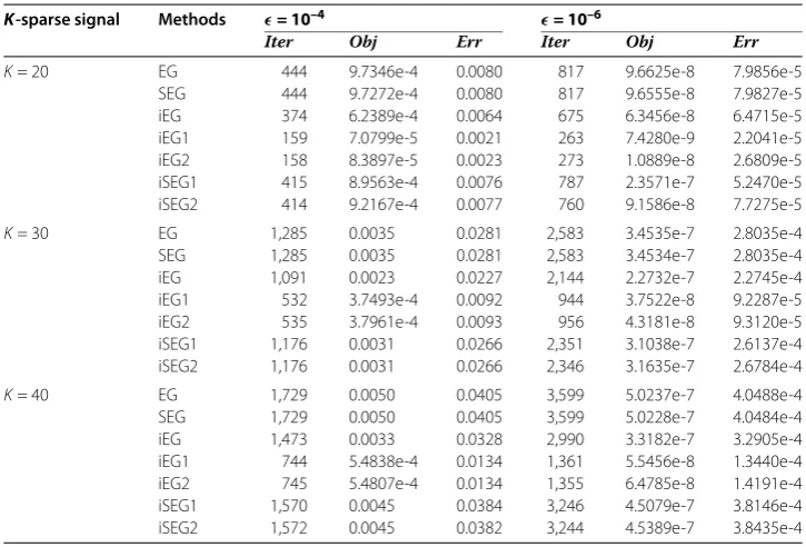
[image:21.595.116.479.487.733.2]the sparse signal from noiseless data b. For the noiseless case, the obtained numerical results are reported in Table . To visually view the results, Figure shows the recovered signal compared with the true signalxwhenK= . We can see from Figure that the
Table 1 Numerical results obtained by the proposed iterative algorithms whenm= 240,
n= 1,024 in the noiseless case
K-sparse signal Methods = 10–4 = 10–6
Iter Obj Err Iter Obj Err
K= 20 EG 444 9.7346e-4 0.0080 817 9.6625e-8 7.9856e-5
SEG 444 9.7272e-4 0.0080 817 9.6555e-8 7.9827e-5
iEG 374 6.2389e-4 0.0064 675 6.3456e-8 6.4715e-5
iEG1 159 7.0799e-5 0.0021 263 7.4280e-9 2.2041e-5
iEG2 158 8.3897e-5 0.0023 273 1.0889e-8 2.6809e-5
iSEG1 415 8.9563e-4 0.0076 787 2.3571e-7 5.2470e-5
iSEG2 414 9.2167e-4 0.0077 760 9.1586e-8 7.7275e-5
K= 30 EG 1,285 0.0035 0.0281 2,583 3.4535e-7 2.8035e-4
SEG 1,285 0.0035 0.0281 2,583 3.4534e-7 2.8035e-4
iEG 1,091 0.0023 0.0227 2,144 2.2732e-7 2.2745e-4
iEG1 532 3.7493e-4 0.0092 944 3.7522e-8 9.2287e-5
iEG2 535 3.7961e-4 0.0093 956 4.3181e-8 9.3120e-5
iSEG1 1,176 0.0031 0.0266 2,351 3.1038e-7 2.6137e-4
iSEG2 1,176 0.0031 0.0266 2,346 3.1635e-7 2.6784e-4
K= 40 EG 1,729 0.0050 0.0405 3,599 5.0237e-7 4.0488e-4
SEG 1,729 0.0050 0.0405 3,599 5.0228e-7 4.0484e-4
iEG 1,473 0.0033 0.0328 2,990 3.3182e-7 3.2905e-4
iEG1 744 5.4838e-4 0.0134 1,361 5.5456e-8 1.3440e-4
iEG2 745 5.4807e-4 0.0134 1,355 6.4785e-8 1.4191e-4
iSEG1 1,570 0.0045 0.0384 3,246 4.5079e-7 3.8146e-4
Figure 1 Comparison of the different methods for sparse signal recovery. (a1)is the true sparse signal,
[image:22.595.119.478.369.571.2](a2)-(a8)are the recovered signals vs the true signal by ‘EG’, ‘SEG’, ‘iEG’, ‘iEG1’, ‘iEG2’, ‘iSEG1’ and ‘iSEG2’, respectively.
Figure 2 Comparison of the objective function value versus the iteration numbers of different methods.
recovered signal is the same as the true signal. Further, Figure presents the objective function value versus the iteration numbers.
Table 2 Numerical results for the proposed iterative algorithms with different noise valueβ
Variances Methods = 10–4 = 10–6
Iter Obj Err Iter Obj Err
β= 0.01 EG 1,264 0.0092 0.0317 2,192 0.0061 0.0131
SEG 1,264 0.0092 0.0317 2,192 0.0061 0.0131
iEG 1,070 0.0081 0.0272 1,812 0.0061 0.0131
iEG1 519 0.0063 0.0164 788 0.0061 0.0130
iEG2 516 0.0063 0.0166 786 0.0061 0.0130
iSEG1 1,156 0.0089 0.0305 1,995 0.0061 0.0131
iSEG2 1,157 0.0089 0.0304 1,990 0.0061 0.0131
β= 0.02 EG 1,274 0.0163 0.0387 2,086 0.0142 0.0272
SEG 1,274 0.0163 0.0387 2,086 0.0142 0.0272
iEG 1,070 0.0154 0.0356 1,728 0.0142 0.0272
iEG1 492 0.0144 0.0300 756 0.0142 0.0272
iEG2 495 0.0143 0.0300 759 0.0142 0.0272
iSEG1 1,163 0.0161 0.0378 1,899 0.0142 0.0272
iSEG2 1,161 0.0161 0.0380 1,895 0.0142 0.0272
β= 0.05 EG 1,190 0.1012 0.0749 1,869 0.0991 0.0651
SEG 1,190 0.1012 0.0749 1,869 0.0991 0.0651
iEG 996 0.1005 0.0727 1,542 0.0991 0.0650
iEG1 460 0.0993 0.0677 670 0.0991 0.0650
iEG2 461 0.0993 0.0675 665 0.0991 0.0650
iSEG1 1,084 0.1010 0.0742 1,704 0.0991 0.0651
[image:23.595.116.478.98.518.2]iSEG2 1,084 0.1010 0.0742 1,704 0.0991 0.0651
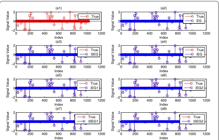
Figure 3 Comparison of the objective function value versus the iteration numbers of different methods in the noise case ofβ= 0.02.
Example . LetF:R→Rbe defined by
F(x,y) =x+ y+sin(x), –x+ y+sin(y), ∀x,y∈R. (.)
The authors [] proved that Fis Lipschitz continuous withL=√ and -strongly monotone. Therefore the variational inequality (.) has a unique solution, and (, ) is its solution.
LetC={x∈R|e
≤x≤e}, wheree= (–, –) ande= (, ). Take the initial
pointx= (–, )∈R. Since (, ) is the unique solution of the variational inequality
Figure 4 Comparison of the different methods for sparse signal recovery. (a1)is the true sparse signal,
(a2)-(a8)are the recovered signals vs the true signal by ‘EG’, ‘SEG’, ‘iEG’, ‘iEG1’, ‘iEG2’, ‘iSEG1’ and ‘iSEG2’ in the noise case ofβ= 0.02, respectively.
Example . LetF:Rn→Rndefined byF(x) =Ax+b, whereA=ZTZ,Z= (zij)n×nand
b= (bi)∈Rn, wherezij∈(, ) andbi∈(, ) are generated randomly.
It is easy to verify thatFisL-Lipschitz continuous andη-strongly monotone withL= max(eig(A)) andη=min(eig(A)).
LetC:={x∈Rn| x–d ≤r}, where the center
d∈(–, –, . . . , –), (, , . . . , )⊂Rn (.)
and radius r∈(, ) are randomly chosen. Take the initial pointx= (ci)∈Rn, where
ci∈[, ] is generated randomly. Setn= . Takeρ= . and other parameters are set the same values as in Example .. Although the variational inequality (.) has a unique solution, it is difficult to get the exact solution. So, denote byDk:=xk+–xk ≤–the stopping criterion.
Figure 5 Comparison of the number of iterations of different methods for Example 6.2.
Figure 6 Comparison of the number of iterations of different methods for Example 6.3.
7 Conclusions
[image:25.595.117.478.331.540.2]Appendix
In this part, we present the details of computing a vectory∈Rnonto the-norm ball
constraint. For convenience, we consider projection onto the unit-norm ball first. Then
we extend it to the general-norm ball constraint.
The projection onto the unit-norm ball is to solve the optimization problem
min
x∈Rn
x–y
s.t. x≤.
The above optimization problem is a typical constrained optimization problem, we con-sider solving it based on the Lagrangian method. Define the Lagrangian functionL(x,λ) as
L(x,λ) = x–y
+λ
x–
.
Let (x∗,λ∗) be the optimal primal and dual pair. It satisfies the KKT conditions of
∈x∗–y+λ∗∂x∗,
λ∗x∗– = ,
λ∗≥.
It is easy to check that ify≤, thenx∗=yandλ∗= . In the following, we assume
y > . Based on the KKT conditions, we obtainλ∗> andx∗= . From the first
order optimality, we havex∗ =max{|y|–λ∗, } ⊗Sign(y), where⊗represents element-wise multiplication and Sign(·) denotes the symbol function,i.e.,Sign(yi) = ifyi≥; otherwiseSign(yi) = –.
Define a functionf(λ) =x(λ), wherex(λ) =Sλ(y) =max{|y|–λ, }⊗Sign(y). We prove
the following lemma.
Lemma A. For the function f(λ),there must existλ∗> such that f(λ∗) = .
Proof Sincef() =S(y)=y> . Letλ+=max≤i≤n{|yi|}, thenf(λ+) = < . Notice thatf(λ) is decreasing and convex. Therefore, by the intermediate value theorem, there
existsλ∗> such thatf(λ∗) = .
To findλ∗such thatf(λ∗) = , we follow the following steps.
Step . Define a vectorywith the same element as|y|, which was sorted in descending
order. That is,y≥y≥ · · · ≥yn≥.
Step . For everyk= , , . . . ,n, solve the equationki=yi–kλ= . Stop search until the solutionλ∗belongs to the interval [yk+,yk].
In conclusion, the optimalx∗can be computed byx∗=max{|y|–λ∗, } ⊗Sign(y). The next lemma extends the projection onto the unit-norm ball to the general-norm ball