Power Control Strategy for Wireless Sensor Networks Based on Cross layer Optimization

14th International Conference on Wireless Communications, Networking and Mobile Computing (WiCOM 2018) ISBN: 978-1-60595-578-0

Power Control Strategy for Wireless Sensor Networks

Based on Cross-layer Optimization

Songhua Hu, Xiaofeng Wang and Yanping Chen1

ABSTRACT

Cross-layer design was proposed in recent years, it was mainly used in network architecture design. Now it is widely introduced in wireless sensor networks. This paper focuses on cross-layer optimization with physical layer, MAC layer and network layer in wireless sensor networks, which is applied to sensor node power control. Based on maximum communication range of sensor nodes, several power control levels are designed. Transmission power of neighbor nodes is classified into different power levels. Neighbor nodes transmit data to central node with designed level of power according to distances. Central node exchanges information with neighbor nodes through cross-layer optimization. Simulation results show that cross-layer optimization for node transmission power control can greatly save node energy consumption, under the condition of nearly same average network throughput with no power control. The most can save energy up to 63.8%.

Keywords: Cross-layer Optimization, Wireless Sensor Networks (WSNs), Power Control, Power Level

INTRODUCTION

Cross-layer optimization is mainly used in wireless network, which is proposed to improve the overall performance of wireless network in recent years [1-3]. Because network resources are very limited, cross-layer optimization is widely applied in the design of algorithms and protocols in WSNs. The goal of cross-layer optimization is to make each layer shared related information with other layers so as to improve the overall performance of network, which is a hot research topic in the field of wireless communication [4-5].

Transmission power control is a typical example of cross-layer design problem [6]. First, because transmission power affects quality of signal, so it affects physical layer. Second, because transmission power determines number of neighboring sensor nodes, which also impacts influence on MAC layer and network layer. Third, transmission power also affects interference caused by congestion, thus it also affects transport layer. At last, transmission power control can also affect network metrics, such as throughput, delay and energy consumption. In this paper, cross-layer optimization is proposed with joint

transmission power control for physical layer, MAC layer and network layer. The key point of this paper

is to adjust network topology by using power control strategy for network layer, to keep number of neighbors to make sure network connectivity and transmit message through MAC layer. During the implementation stage, with different power control strategy in network layer, power control in MAC layer and physical layer make adjustment in a TDMA time slot. By decreasing the energy consumption of

1 _{Department of Computer Science and Technology, Hefei University, Hefei, 230601, People’s Republic of China}

sensor nodes, transmission power control reduces energy consumption of the whole network, so it prolongs the lifetime of WSNs.

SYSTEMMODEL

A. Network Model

For small scale of WSNs, typical network architecture is shown in Fig.1. Sink node is located in a corner of the rectangular monitoring area, sensor nodes are randomly distributed in the monitoring area. Monitoring data will be sent to sink from sensor nodes using multi-hop communication mode through the relay nodes. Therefore, sensor nodes near to sink consume more energy because they relay data packets [7]. Besides sink nodes, sensor nodes are with the same hardware structure, so transmission power control of sensor nodes becomes extremely important.

Sensor Nodes

Figure 1. WSNs structure in monitoring area .

B. Multiple time slots for transmission scheme

Because sensor nodes will lead to conflict if they transmit simultaneously, so transmission mode is adopted in MAC layer by time slots. It allows each node owning a time slot for transmission. Assuming

that there are n sensor nodes in WSNs, a CDMA period of Tis divided intontime slots according to n

sensor nodes，every node, denoted as

i

n ,occupying a t_i for transmission, so, for i1, 2, n,



transmission rate should be less than data transmission rate limit determined by Shannon theorem. Therefore, According to allocate different time slots for sensor nodes dynamically, which can make data transmission rate of each node as large as possible, so the overall network throughput can achieve better results.

C. Transmission power control strategy

According to Leach in [8], a metric round is defined within a CDMA periodT. In initialization stage of

network, each sensor node sends SYNC packet to neighbor nodes with maximum power. We make an

assumption that a node i, sensor node i calculates the received signal power according to RSSI signal

minimum power threshold asPr_threshold, so transmission power Pti_min of node i can be calculated as

follows:

_ min _ , 1, 2,

ti

ti r threshold ri

P

P P i n

P

   (1)

Where

ri ti

P P

can be got by (2), so,P_{ti_ min},i1, 2, n is minimum transmission power.

L d G G P

P t t r

r 2 2

2

) 4

( 



 (2)

Formula (2) is Friis formula of free space propagation loss when waves transmission, here, P_t is

transmission power, P_ris receiver power, G_tand G_rare defined as antenna gain for sender and receiver

respectively; is a wavelength; dis the distance between sender and receiver, L is System loss factor,

1 L .

Because sensor nodes transmits data packets to sink in a multi-hop transmission mode, so power control strategy can be summarized as: for an arbitrary sensor nodes, searching for the optimization of

_ min

,

ti ti ti tn

P P  P  P ,i1, 2, n, here, P_tnis maximization transmission power of sensor nodes.

Because of sensor nodes from different manufacturers with different functions, we assume only one type of sensor node. So transmission power can be divided into X levels, if maximum communication radius

is R, each sensor node can take itself as center node, so it’s nearby area is divided into equally spaced

annular region, the radius of annular region can be expressed as (3):

R r

X

 (3)

For sensor node i, its neighbor nodes are distributed in numbers of X inner annular region, with radius

of kr (k 1, 2, X) from near to far. If defined d as distance between a neighbor node and sensor node

i, d can be expressed as:

,

d krb br (4)

If distance is d, transmission power P_ti of neighbor nodes of node i can be selected with the following

formula:

1 2

{ , , } 1, 2, ,

ti t t tX

P  P P P i X (5)

Here,Pt1 Pti_min。

CROSS-LAYEROPTIMIZATIONSTRATEGY

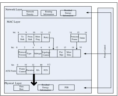
ACK Frame P o w er C o n tr o l 16

8 9 10 11 12

To Sink From Sink More Frag Retry 14 15 Protected Frame Order bit:

0 16 32 80 112 Frame

ControlDuration RA FCS bit:

bit: 0 2 4 6 8 12 13 14 16

Protocol VersionType Subtype

Pwr Mgt More Data Topology Control Network Layer MAC Layer

Physical Layer

Network Density Routing Information Residual Energy Information Data Rate Residual Energy Information PER

Figure 2. Cross-layer information sharing in three layers.

A. Processing of energy information through across-layer

Residual energy information can be got and updated by cross-layer report function and ACK frame. Compared with the existing algorithms, it avoids the special bits of information, thus it saves the node energy and bandwidth, and the details are as follows:

(1)Residual energy of sensor nodes is measured in it’s time slots in physical layer, then energy information is reported to MAC layer and network layer through cross-layer report function, then residual energy information is updated.

(2) When sensor node receives data packets from others, it answers ACK frame to them. If residual energy satisfies the classification of energy level, residual energy information is packaged into ACK frame and sent to each other, as shown in Fig. 2.

(3) When sensor node receives the ACK frame, it gets the information To sink. As shown in Fig.2, Frame field includes these fields, such as More Fragments, Retry, Protected, Frame, Order from. Sensor nodes gets the residual energy information of these fields, thus they updates the routing table in network layer, then it revert the default values of these fields as 0.

B. Energy-saving mechanism combined with RSSI and power control

In this paper, energy-saving mechanism combined with RSSI and power control is designed. The basic idea is got the distance between sensor nodes by RSSI information. Sensor node adjusts transmission power during packet transmission process according to distance between each other, which avoids using maximum transmission power all the time, thereby it saves energy. The details are as follows:

(1)When sensor node receives packets, the transmission power value is reported from physical layer to network layer by cross-layer information. Network layer information of sensor nodes calculates distance between sensor nodes and other neighboring nodes and stores distance information in neighbor distance table.

(2)When node i transmits a packet to the neighbor node j , the first step is identifying the distance d_ij

in neighbor distance table, then determines the transmission power from the table “distance - transmission power”, and sends the transmission power value to physical layer, so the transmission

power is adjusted and packets are sent to node j.

Sink node creates the whole network broadcast uplink routing packets by Flooding mode. The information are node ID, node hops from sink to node and node residual energy, which can get in the packets. When sensor node receives uplink routing packets, sensor node gets the routing gradient from sink to itself according to the obtained information, then uplink routing is established. The specific steps are as follows:

(1)In initialization phase, number of hops (TTL) of sink is set to 0, number of hops of other nodes (TTL) is set to infinity. Sink node creates uplink routing packets with broadcast mode with the communication

radiusR.

(2)When sensor node i receives the uplink routing packets from node n , it calculates the distance

in

d with node nbased on the RSSI information and stored the information in table of neighbor distance,

then it creates the routing packets with the following procedure: (a) if TTLi TTLn1, then it sets

1

i n

TTL TTL  , clears the existing uplink routing table, stores information of node ID，TTLn and

residual energy. Then sensor node i creates the corresponding uplink routing packet of its own and

broadcasts the information to the neighbor node. (b) if TTL_i TTL_n 1,then sensor node i only adds

nodes ID in upstream routing table, while TTL_nand residual energy are discarded from uplink routing

packet. (c) if TTL_i TTL_n1, no uplink routing packet is created and nothing is done.

 Downlink routing

Source routing mode is applied in downlink routing, without special control packet, thus it reduces the network overhead. The specific steps are as follows:

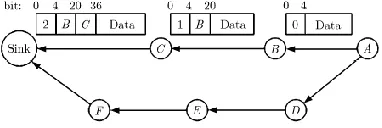
(1) In first control packet sent to sink, each sensor node creates a predetermined and changeable relay routing table according to the its own gradients. When packet is sent and relay routing, it records node ID, hops information, as shown in Fig.3.

Figure 3. Routing information from sensor node to Sink.

(2) When sensor node receives first data packet from other nodes, it judges whether sends or relays data packet. If it receives, it gets the data packet header from routing table, then it updates its downlink routing table.Also it writes its own ID into routing table and update the routing table information of relay hops. Then the packet is sent to the next node,if it isn’t, it only updates its own routing table and relay hops. It sends data packet to the next hop node. If a sensor node does not send or relay any data packets in predefined time, then it sends a data packet without useful data the sink.

(3) In uplink data packet transmission process, when sensor node receives the data packet, it checks the packet header information whether there is downlink routing in routing table or a data source node Routing.If it is a downlink routing, then it updates the routing; otherwise, it sets up a routing to data source node in downlink routing table.

 Data packet transmission

It it the criteria that numbers of hops and residual energy is used in data packets transmission in uplink and downlink routing. In the basis of hops as a priority, sensor node which has more residual energy is

put forwarded, where TTL_c is the hops from sensor node to sink, E_r and E_i is residual energy and

initial energy of sensor node respectively. BecauseE_i E_r 0, so

1

c c c

TTL H TTL  (6)

When selecting the next hop, the smallest value of H_c in neighboring senor node is selected. From (6),

we can draw the conclusion that the probability of node is selected as next hop when it has more residual

energy and smaller synthesis hopsH_c, which helps to achieve balance between nodes and extends the

network lifetime. When a sensor node has a packet to transmit, it checks its own routing table, then it

finds the minimum number of synthesis hops H_cof nodes (if it is j), and also it finds the real distance

ij

d according distance routing table in neighbor nodes, then it adjusts the transmit power, then it sends

the packet to sensor node jwith it.

NUMERICALSIMULATIONS

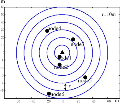
Make an assumptions that power levels of a sensor node is 6, ifX 6, according to references [12-15],

in order to improve the channel utilization and maximize the network throughput, the optimal number of neighbor nodes is set to 6~8. We now set the number is 6, and also set maximum communication radius of sensor node is 60m. So every sensor node and its neighbor nodes can be divided into several rings of node distribution, as shown in Fig.4.

In NS2, sensor nodes with power control and without power control are compared from energy consumption, packet loss rate, delay and throughput. In experiment, the experiment setting as as follows: sensor nodes is organized by multi-hop network, it uses direct sequence spread spectrum (DSSS) technology in physical layer, bandwidth is 2 Mbps, bit stream is CBR (const bit rate) in application layer, UDP protocol is used in transport layer, routing protocol is AODV, nodes are static distribution, sensor node number is 7, center sensor node receives data packets from neighboring nodes, the other 6 neighboring nodes are randomly distributed in 6 concentric rings with the central node as the center of

the circle, concentric interval is set to r10m.

As shown in Fig.4, the range of 60m is divided into 10m, 20m, 30m, 40m, 50m, 60m. According to

formula (2), makeL1,G_t 1,G_r 1,H_t H_r 1.5m, the frequency of transmitting wave is 9.14 10 8,

-60 -40 -20 0 20 40 60 -50

-40 -30 -20 -10 0 10 20 30 40 50 60

m r=10m

r node1

node3 node4

node2

node5

node6 m

Figure 4. Sensor nodes distribution.

TABLE 1.RELATIONSHIP BETWEEN MINIMUM TRANSMISSION POWER AND

DISTANCE OF NODES (MAXIMUM COMMUNICATION RADIUS R=60M).

Distance between nodes（m）

Minimum transmission power Pt_min(w)

Received power

threshold(dB)

10 0.0078 -72.7

20 0.0313 -72.7

30 0.0704 -72.7

40 0.1251 -72.7

50 0.1955 -72.7

60 0.2818 -72.7

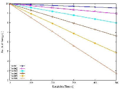
Parameter settings in NS2 simulation is shown in Tab.2. After 500s of simulation, comparisons of residual energy and energy saving ratio between without transmission power control and based on cross-layer optimization transmission power control are shown in Tab.3. It can be seen from the table that the most of energy saving ratio which is based on cross-layer power transmission control can save energy up to 68.3%. At the same time, the relationship between residual energy of nodes with simulation time is shown in Fig.5. As can be seen from the figure that if it is the nearest distance, the most can save energy. With simulation time goes, the trend is getting better and better.

TABLE 2.PARAMETER SETTINGS IN NS2 SIMULATION.

Parameter Value

Network area size

(m2)

3600

Number of nodes 7(1 core node ,6 sensors

Traffic type CBR(time:1s-500s, packetSize:512bit,

interval:0.1s) Number of transmit

power levels

6

Network Initial Energy(J)

10

Power for reception (Watt)

0.001

Power for idle (Watt) 0.0005

Power for sleep (Watt) 0

Power for sleep/idle transition (Watt)

0.0001

Time for sleep/idle transition (s)

0.005

Ranges corresponding to the power levels

10m,20m,30m,40m, 50m

，60m

Simulation time 500s

TABLE 3.RESIDUAL ENERGY OF SENSOR NODES (JOULE).

Nodes

Without power control

Cross-layer optimization power control

energy saving ratio

Node1 2.727446 9.566310 68.3%

Node

2 2.727446 8.979765 62.5%

Node

3 2.727446 8.003854 52.7%

Node

4 2.727446 6.638577 39.1%

Node

5 2.727446 4.881438 21.6%

Figure 5. Residual energy of sensor nodes.

CONCLUSIONS

The main work of this paper is study of cross-layer optimization for transmission power control between physical layer, MAC layer and network. According to maximum communication radius of sensor nodes, transmission power of sensor nodes is divided into several power levels according to the distance. Sensor nodes choose optimism transmission power to sends data to their neighboring nodes. This paper gives the detail calculation of power selection, routing selection of cross-layer optimization. Simulation results show that the proposed cross-layer power control strategy can greatly reduce energy consumption, improve network throughput and also have a good guiding significance for optimization of WSNs. In next step of work, in order to improve the network performance, we will consider flow control of transport layer which is introduced to cross-layer power control.

ACKNOWLEDGMENT

The authors would like to thank the anonymous reviewers and editors for their valuable comments. The material presented in this paper is supported by the grant of the National Natural Science Foundation of China, No. 61672204, the grant of Major Science and Technology Project of Anhui Province, No. 17030901026, the grant of Key Constructive Discipline Project of Hefei University, No. 2016xk05,the grant of Natural Science Fund Project of Anhui Province, No. KJ2018A0557,This study was supported by Anhui Province Key Laboratory of Industry Safety and Emergency Technology,No.ISET201809,the grant of Talent Fund Project of Hefei University ,No.16-17RC17.

REFERENCES

[1] Melodia T., M. Vuran, D. Pompili. The state of the art in cross-layer design for wireless sensor networks.Wireless Systems and Network Architectures in Next Generation Internet, 2006:78-92.

[3] Lin X., N. Shroff, R. Srikant. A tutorial on cross-layer optimization in Wireless networks. IEEE Journal on Selected Areas in Communications, 2006, 24(8): 1452-1463.

[4] Attarkashani A, Hamouda W, Attarkashani A, et al. Throughput maximization using cross-layer design in wireless sensor networks[C]// ICC 2017 - 2017 IEEE International Conference on Communications. IEEE, 2017:1-6.

[5] Shakkottai S, Rappaport T S, Karlsson P C. Cross-layer design for wireless networks. IEEE Transactions on Communications, 2003, 41(10): 74-80.

[6] Hu S, Han J. Power control strategy for clustering wireless sensor networks based on multi-packet reception[J]. Wireless Sensor Systems let, 2014, 4(3):122-129.

[7] Ranjan R, Varma S. Challenges and Implementation on Cross Layer Design for Wireless Sensor Networks[J]. Wireless Personal Communications, 2016, 86(2):1-24.

[8] Heinzelman W, Chandrakasan A, Balakrishnan H. Energy-Efficient communication protocol for wireless micro sensor networks. In: Proc. of the 33rd Annual Hawaii Int. Conf. on System Sciences. Maui: IEEE Computer Society, 2000, pp. 3005-3014.

[9] Lin S, Zhang JB, Zhou G, Gu L, He T, Stankovic A. ATPC: Adaptive transmission power control for wireless sensor networks. In Proc. of the Sensys 2006. Boulder: ACM Press, 2006, pp. 223−236.

[10] Dobslaw F, Zhang T, Gidlund M. QoS-Aware Cross-Layer Configuration for Industrial Wireless Sensor Networks[J]. IEEE Transactions on Industrial Informatics, 2016, 12(5):1679-1691.

[11] J. Yuan, Z. Li, W. Yu, B. Li. A Cross-Layer optimization framework for multicast in multi-hop wireless networks wireless internet. In Proc. WICON ’05, July, 2005, pp.47–54.

[12] Yu CS, Shin KG, Lee B. Power-Stepped protocol: Enhancing spatial utilization in a clustered mobile ad hoc network. IEEE Journal on Selected areas in communications, 2004, 22(7):1322−1334.

[13] Kurt S, Yildiz H U, Yigit M, et al. Packet Size Optimization in Wireless Sensor Networks for Smart Grid Applications[J]. IEEE Transactions on Industrial Electronics, 2017, PP(99):1-1.

[14] Alshinina R, Elleithy K. Performance and Challenges of Service-Oriented Architecture for Wireless Sensor Networks[J]. Sensors, 2017, 17(3):536-575.